Meta-analysis on the OTIM-DB
The meta-analysis will focus on the effect of land use, tillage, compaction and sampling time on the hydraulic conductivity.
import numpy as np
import pandas as pd
import matplotlib.pyplot as plt
import seaborn as sns

datadir = '../data/'
outputdir = '../figures/'
letters = ['a','b','c','d','e','f','g','h','i','j','k','l','m','n','o','p','q','r','s','t','u','v']
# read in database
dfdic = pd.read_excel(datadir + 'OTIM-DB.xlsx', sheet_name=None, na_values=[-9999])
dfexp = dfdic['experiments']
dfloc = dfdic['locations']
dfref = dfdic['reference']
dfmeth = dfdic['method'].replace(-9999, np.nan)
dfsp = dfdic['soilProperties']
dfclim = dfdic['climate']
kcols = ['k{:d}'.format(i+1) for i in range(10)]
dfmod = dfdic['modelFit'].rename(columns=dict(zip(kcols, [a.upper() for a in kcols])))
dfsm = dfdic['soilManagement'].replace(-9999, np.nan).replace(
'no impact', 'consolidated').replace( # estetic replacement
'after tillage', 'soon after tillage')C:\Users\gblanchy\WPy64-3890\python-3.8.9.amd64\lib\site-packages\openpyxl\worksheet\_reader.py:312: UserWarning: Unknown extension is not supported and will be removed
warn(msg)
C:\Users\gblanchy\WPy64-3890\python-3.8.9.amd64\lib\site-packages\openpyxl\worksheet\_reader.py:312: UserWarning: Conditional Formatting extension is not supported and will be removed
warn(msg)
Check indexes
Check that all indices are unique in each table.
# check indexes are unique
indexes = [
    ('experiment', dfexp, 'MTFName'),
    ('location', dfloc, 'Location'),
    ('reference', dfref, 'ReferenceTag'),
    #('methodTargetFit', dfmtf, 'MTFName'),
    #('soilSiteProperties', dfssp, 'SSPName'),
    ('method', dfmeth, 'MethodName'),
    ('soilProperties', dfsp, 'SPName'),
    ('climate', dfclim, 'ClimateName'),
    ('modelFit', dfmod, 'MTFName'),
    ('soilManagement', dfsm, 'SMName'),
]
for name, df, col in indexes:
    a = df[col].unique().shape[0]
    b = df.shape[0]
    c = 'ok' if a == b else 'not ok => indexes are not unique!'
    print('{:20s}: {:5d} rows with {:5d} unique values: {:s}'.format(name, a, b, c))
experiment : 1297 rows with 1297 unique values: ok
location : 205 rows with 205 unique values: ok
reference : 172 rows with 172 unique values: ok
method : 1297 rows with 1297 unique values: ok
soilProperties : 1297 rows with 1297 unique values: ok
climate : 205 rows with 205 unique values: ok
modelFit : 1297 rows with 1297 unique values: ok
soilManagement : 1297 rows with 1297 unique values: ok
# check indexes are all specified (intersection with 'experiment' tab)
for name, df, col in indexes[1:]:
    a = df[col]
    b = dfexp[col]
    ie1 = a.isin(b)
    ie2 = b.isin(a)
    c = 'not ok, some indexes are missing from experiment or ' + name
    if (np.sum(~ie1) == 0) & (np.sum(~ie2) == 0):
        c = 'ok'
    else:
        miss1 = ', '.join(a[~ie1].tolist()) + ' only in ' + name
        miss2 = ', '.join(b[~ie2].tolist()) + ' only in experiment'
        c = 'not ok\n\t' +  miss1 + ';\n\t' + miss2
    print('{:20s} contains {:3d} not related rows, experiment: {:3d} => {:s}'.format(
        name, np.sum(~ie1), np.sum(~ie2), c))
location contains 0 not related rows, experiment: 0 => ok
reference contains 0 not related rows, experiment: 0 => ok
method contains 0 not related rows, experiment: 0 => ok
soilProperties contains 0 not related rows, experiment: 0 => ok
climate contains 0 not related rows, experiment: 0 => ok
modelFit contains 0 not related rows, experiment: 0 => ok
soilManagement contains 0 not related rows, experiment: 0 => ok
Filtering entries and aggregation
Entries are kept if:
- they come from topsoil:
UpperD_m< 0.2 m - are well fitted:
R2> 0.9 - measure the full range from 0 mm to 100 mm tension:
Tmax>= 100 mm andTmin== 0 mm
Entries are aggregated (averaged) if they do no differ according to the columns chosen. Then, all entries aggregated are considered replicates and a standard error is estimated if more than one entries is aggregated.
Knowing the SD for each paired comparison is quite difficult in our case as often single mean values are reported and error bars in log graph are inconsistents. To estimate an SD when it's not reported, multiple methods can be used, see:
Wiebe, Natasha, Ben Vandermeer, Robert W. Platt, Terry P. Klassen, David Moher, and Nicholas J. Barrowman. 2006. “A Systematic Review Identifies a Lack of Standardization in Methods for Handling Missing Variance Data.” Journal of Clinical Epidemiology 59 (4): 342–53. https://doi.org/10.1016/j.jclinepi.2005.08.017.
In our case, we use a two steps process:
- for paired comparison with multiple replicates, we estimate the SD based on the SD of the ES of the replicates within the same study (during aggregation process)
- if there is only one replicate, then we use the CV accross all similar paired comparison from all studies and back-compute the SD with:
# merge tables
# NOTE good to merge on specific column (in case same column name appears...)
dflu = dfexp.merge(
    dfloc, how='left', on='Location').merge(
    dfref, how='left', on='ReferenceTag').merge(
    dfmeth, how='left', on='MethodName').merge(
    dfsp, how='left', on='SPName').merge(
    dfclim, how='left', on='ClimateName').merge(
    dfmod, how='left', on='MTFName').merge(
    dfsm, how='left', on='SMName')
dflu = dflu[dflu['ReferenceTag'].ne('kuhwald2017')].reset_index(drop=True)  # remove this entry as only one tension
print('number of entries (rows) initially in the db (as reported in papers):', dflu.shape[0])

# remove entries with R2 lower than 0.9
dflu = dflu[dflu['R2'].ge(0.9)].reset_index(drop=True)
print('number of entries with R2 >= 0.9:', dflu.shape[0])

# remove entries that do not go up to 100 mm tension
ifull = dflu['Tmax'].ge(100) & dflu['Tmin'].le(0)
dflu = dflu[ifull].reset_index(drop=True)
print('number of entries with Tmax >= 100 mm:', dflu.shape[0])

# removing subsoil data
isub = dflu['UpperD_m'].lt(0.2)
dflu = dflu[isub].reset_index(drop=True)
print('number of entries with UpperD < 0.2 m (topsoil):', dflu.shape[0])

# saving
dflu.to_csv(datadir + 'dfotimd.csv', index=False)
number of entries (rows) initially in the db (as reported in papers): 1285
number of entries with R2 >= 0.9: 1183
number of entries with Tmax >= 100 mm: 443
number of entries with UpperD < 0.2 m (topsoil): 409
# distribution of number of entries per paper
s = dflu['ReferenceTag'].value_counts()
display(s)
fig, ax = plt.subplots(figsize=(14, 2))
s.plot.bar(ax=ax)
Alletto_2009_G 36
Schwen_2011_SaTR 27
Fuentes_2004_SSSoAJ 25
Zhang2016 24
Zhou_2008_C 24
..
Moosavi_2012_AAaSS 1
Schwarzel_2007_SSSoAJ 1
Timlin_1994_SSSoAJ 1
Carey_2007_HP 1
Moreno_1995_AaWM 1
Name: ReferenceTag, Length: 61, dtype: int64<AxesSubplot:>
# number of time measurement per paper
sdf = dflu.groupby(['ReferenceTag', 'Month1', 'Month2', 'YearExp']).count().reset_index()
s = sdf['ReferenceTag'].value_counts()
display(s)
fig, ax = plt.subplots(figsize=(14, 2))
s.plot.bar(ax=ax)
Bodner2013 12
Schwen_2011_SaTR 10
Fuentes_2004_SSSoAJ 6
Zhang2016 6
Zeng2013 5
Cameira_2003_SaTR 5
Hu_2009_G 4
Alletto_2009_G 3
Zeinalzadeh_2011_JoFAaE 3
Moret_2007_SaTR 3
Coquet_2005_G 3
Frey_2012_SSSoAJ 3
Reynolds_1995_SaTR 2
Moreno_1997_SaTR 2
Wu_1992_SaTR 2
Zhou_2008_C 2
Miller2018 2
Asada_2012_EJoSS 2
Shouse_1998_WRR 1
Schwen_2011_SSSoAJ 1
Carey_2007_HP 1
Bodhinayake_2004_HP 1
Ankeny_1990_SSSoAJ 1
Bagarello_2007_G 1
Moret_2007_SSSoAJ 1
kelishadi2014 1
Spongrova_2009_VZJ 1
Mandal_2005_JoISSS 1
Sanou_2010_SUaM 1
Angulo-Jaramillo_1996_SSSoAJ 1
Timlin_1994_SSSoAJ 1
khetdan2017 1
kabir2020 1
Coutadeur_2002_AiG 1
Coutadeur_2002_EJoSS 1
zeng2013b 1
Lampurlanes_2006_SaTR 1
Trojan_1998_SSSoAJ 1
Mohanty_1994_WRR 1
Name: ReferenceTag, dtype: int64<AxesSubplot:>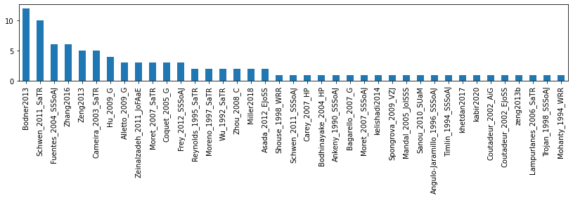
# create classes
print('number of rows after filtering: {:d} ({:d} studies)'.format(
    dflu.shape[0], dflu['ReferenceTag'].unique().shape[0]))

# create classes to enable to average on them
dflu['BulkDensityClass'] = pd.cut(dflu['BulkDensity'], bins=[0, 1, 1.2, 1.4, 1.6, 2]).astype(str)
dflu['BulkDensityClass'] = dflu['BulkDensityClass'].astype(str)  # to set the NaN as 'nan' string
dflu['SoilOrganicCarbonClass'] = pd.cut(dflu['SoilOrganicCarbon'], bins=[0, 0.01, 0.02, 0.03, 0.04, 2]).astype(str)
dflu['SoilOrganicCarbonClass'] = dflu['SoilOrganicCarbonClass'].astype(str)  # to set the NaN as 'nan' string
dflu['AnnualPrecipitationClass'] = pd.cut(dflu['AnnualPrecipitation'], bins=[0, 500, 1000, 1500, 2000, 4000]).astype(str)
dflu['AnnualPrecipitationClass'] = dflu['AnnualPrecipitationClass'].astype(str)
dflu['AnnualMeanTemperatureClass'] = pd.cut(dflu['AnnualMeanTemperature'], bins=[0, 5, 10, 15, 20, 30]).astype(str)
dflu['AnnualMeanTemperatureClass'] = dflu['AnnualMeanTemperatureClass'].astype(str)
number of rows after filtering: 409 (61 studies)
# dfg = dflu.groupby(practices)
# for name, group in dfg:
#     if group.shape[0] > 1:
#         dflu.loc[group.index, 'SD'] = 1
# average studies which do not differentiate according to the columns of interest (aggregation)
practices = [
'LanduseClass',
'TillageClass',
# 'NbOfCropRotation', # not considered because too few studies
# 'ResidueClass',
# 'GrazingClass',
# 'IrrigationClass',
'CompactionClass',
'SamplingTimeClass',
'SoilTextureUSDA',
#'SoilTypeClass',
#'AridityClass', # proxy for climate
'AnnualPrecipitationClass',
'AnnualMeanTemperatureClass',
'BulkDensityClass',
'SoilOrganicCarbonClass',
]
def mode(x):
# most frequent class
return x.value_counts(dropna=False).index[0]
# define the operation to be applied on each group
# mean for numeric column, mode for categorical column
dic = {} # column : function to be applied on the group
colmean = dflu.columns[dflu.dtypes.ne('object')].tolist()
dic.update(dict(zip(colmean, ['mean']*len(colmean))))
colmode = dflu.columns[dflu.dtypes.eq('object')].tolist()
dic.update(dict(zip(colmode, [mode]*len(colmode))))
# for some numeric columns, we just want the sum or the mode, not the mean
dic['Reps'] = 'sum'
for practice in practices:
dic.pop(practice)
dic.pop('ReferenceTag')
# grouping
dfg = dflu.groupby(['ReferenceTag'] + practices)
df1 = dfg.agg(dic).reset_index()
df2 = dfg.sem().reset_index() # compute SD from "replicates"
kcols = ['Ks'] + ['K{:d}'.format(a) for a in range(1, 11)]
df = pd.merge(df1,
df2[['ReferenceTag'] + practices + kcols],
on=['ReferenceTag'] + practices,
suffixes=('', '_sem')).reset_index()
print('reduction in rows after grouping:', dflu.shape[0], '->', df.shape[0],
'({:d} studies)'.format(df['ReferenceTag'].unique().shape[0]))
# detecting entries that only contain one row (so not to be used in meta-analysis
# as no paired comparison is possible)
print('number of studies with only one row (useless for meta-analysis, removed):',
df['ReferenceTag'].value_counts().le(1).sum(), 'studies')
s = df['ReferenceTag'].value_counts().gt(1)
moreThanOneRow = s[s].index.tolist()
df = df[df['ReferenceTag'].isin(moreThanOneRow)].reset_index(drop=True)
print('total number of rows after removing the reference with only one row:', df.shape[0],
'({:d} studies)'.format(df['ReferenceTag'].unique().shape[0]))
dflu = df
# it's very difficult to estimate the standard error after aggregation as we often end-up with
# one row per unique combination
# saving
dflu.to_csv(datadir + 'dfotimd-averaged.csv', index=False)reduction in rows after grouping: 409 -> 193 (61 studies)
number of studies with only one row (useless for meta-analysis, removed): 20 studies
total number of rows after removing the reference with only one row: 173 (41 studies)
(dflu['SD'].notnull() | dflu['K10_sem'].notnull()).sum()84Create pairwise comparision
Inside same study, create pairwise comparison with a control value vs other values.
The control values are given a negative number (-1) and the treatment values a positive number (+1). Several treatment values can be compared against the same control. 0 is when the row is not relevant for the comparison.
# let's replace all 'non' arable by 'not arable' so we can use it as control
dflu['LanduseClass'] = dflu['LanduseClass'].replace(
    {'grassland': 'not arable',
     'woodland/plantation': 'not arable',
     'bare': 'not arable'})
# define controles and their values
controls = [ # column, control, column for pairwise
('LanduseClass', 'not arable', 'pcLanduse'),
('TillageClass', 'no tillage', 'pcTillage'),
#('NbOfCropRotation', 1, 'pcCropRotation'),
#('ResidueClass', 'no', 'pcResidues'),
#('GrazingClass', 'no', 'pcGrazing'),
#('IrrigationClass', 'rainfed', 'pcIrrigation'),
('CompactionClass', 'not compacted', 'pcCompaction'),
('SamplingTimeClass', 'consolidated', 'pcSamplingTime'),
]
# replacements to have more homogenized data
# dflu['ResidueClass'] = dflu['ResidueClass'].replace({'no (exact)': 'no'})
# dflu['PastureClassGrazing'] = dflu['PastureClassGrazing'].replace({'no (excat)': 'no'})
# dflu['IrrigationClass'] = dflu['IrrigationClass'].replace({'no': 'rainfed', 'no (exact)': 'rainfed', 'yes': 'irrigated'})
# dflu['CompactionClass'] = dflu['CompactionClass'].replace({'no ':'no', 'inter-row': 'no', 'no (exact)': 'no'})
# for easier interpretation, we regroup 'after compaction' to 'unknown'
dflu['SamplingTimeClass'] = dflu['SamplingTimeClass'].replace('after compaction', 'unknown')
# reps which are nan are set to 1
print('Number of Reps which are NaN or 0 (replaced by 1):', dflu['Reps'].isna().sum() + dflu['Reps'].eq(0).sum())
dflu['Reps'] = dflu['Reps'].replace(0, np.nan).fillna(1)
# unique values per control
for a, b, c in controls:
print(a, '=>', dflu[a].dropna().unique())Number of Reps which are NaN or 0 (replaced by 1): 2
LanduseClass => ['arable' 'not arable' 'unknown']
TillageClass => ['conventional tillage' 'reduced tillage' 'no tillage' 'unknown']
CompactionClass => ['unknown' 'compacted' 'not compacted']
SamplingTimeClass => ['consolidated' 'soon after tillage' 'unknown']
# build pair-wise comparison
for a, b, c in controls:
    dflu[c] = 0

# columns that should be similar
cols = np.array(['LanduseClass', # often landuse will change with tillage and crop rotation
                 'TillageClass',
                 #'NbOfCropRotation',
                 #'Crop_class',
                 #'Crop Rotation',
                 #'Covercrop_class',
                 #'ResidueClass',
                 #'GrazingClass',
                 #'IrrigationClass',
                 'CompactionClass',
                 'SamplingTimeClass',
                 #'amendment_class',
                 # measurement date/month
                ])

colsdic = {
    'LanduseClass': cols[5:],
    'TillageClass': cols,
    #'NbOfCropRotation': cols,
    #'ResidueClass': cols,
    #'GrazingClass': cols,
    #'IrrigationClass': cols,
    'CompactionClass': cols,
    'SamplingTimeClass': cols,
}

# build pairwise inside each publication
for pub in dflu['ReferenceTag'].unique():
    ie = dflu['ReferenceTag'] == pub
    irows = np.where(ie)[0]
    for ccol, cval, pcColumn in controls:
        c = 0
        cols = colsdic[ccol]
        colSame = cols[cols != ccol].copy()
        #print('pub==', pub)
        for i in irows:
            row1 = dflu.loc[i, colSame]
            inan1 = row1.isna()
            # if the columns is a controlled value
            if dflu.loc[i, ccol] == cval:
                flag = False
                c = c + 1
                for j in irows:
                    if ((j != i) & (dflu.loc[j, ccol] != cval) &
                       (pd.isna(dflu.loc[j, ccol]) is False) &  # not Nan
                       (dflu.loc[j, ccol] != 'unknown')):  # not unknown
                        row2 = dflu.loc[j, colSame]
                        inan2 = row2.isna()
                        #if cval == 'rainfed':
                            #print('1-', pub, row1.values)
                            #print('2-', pub, row2.values)
                        if row1.eq(row2)[~inan1 & ~inan2].all():
                            dflu.loc[i, pcColumn] = -c
                            dflu.loc[j, pcColumn] = c
                            #if cval == 'rainfed':
                           #     print('ok')

for a, b, c in controls:
    print(c, np.sum(dflu[c] > 0))
dflu.to_excel(datadir + 'dflu.xlsx', index=False)
pcLanduse 24
pcTillage 32
pcCompaction 8
pcSamplingTime 12
# number of ES per study (to make sure one study doesn't have too many ES)
# for col in cols:
#     dflu['one'] = dflu['pc' + col.replace('Class', '')].gt(1)
#     print(dflu['one'].sum())
#     df = dflu.groupby('ReferenceTag').count().reset_index().sort_values('one', ascending=False)[['ReferenceTag', 'one']]
#     df.plot.hist(bins=np.arange(1, df['one'].max()+1), title=col)
Effect sizes
Effect sizes (ES) are computed according to this formula:
with as:
For easier interpretation, we can convert back to a change in percent:
If the effect size is greater than 0, that means the treatment is larger than the control.
The weighted mean is computed as:
And the weighted variance of the mean as:
and the standard error of the mean:
# compute effect sizes
kcols = ['Ks'] + ['K{:d}'.format(a) for a in range(1, 11)]
esColumns = ['es' + a[2][2:] for a in controls]
for c in esColumns:
    dflu[c] = np.nan
for pub in dflu['ReferenceTag'].unique():
    ie = dflu['ReferenceTag'] == pub
    for ccol, cval, pcColumn in controls:
        esColumn = 'es' + pcColumn[2:]
        for i in range(np.sum(ie)):
            ieTrt = dflu[pcColumn] == (i+1)
            itrts = np.where(ie & ieTrt)[0]
            if len(itrts) > 0:
                ieCtl = dflu[pcColumn] == -(i+1)
                ictl = np.where(ie & ieCtl)[0][0]
                mtfNameCtl = dflu[ie & ieCtl]['SMName'].values[0]
                controlValues = dflu[ie & ieCtl][kcols].values[0, :]
                controlReps = dflu[ie & ieCtl]['Reps'].values[0]
                for itrt in itrts:
                    mtfNameTrt = dflu.loc[itrt, 'SMName']
                    treatmentValues = dflu.loc[itrt, kcols].astype(float).values
                    treatmentReps = dflu.loc[itrt, 'Reps']
                    escols = [esColumn + '_' + a for a in kcols]
                    dflu.loc[itrt, escols] = np.log10(treatmentValues/controlValues)  # effect size
                    #dflu.loc[itrt, escols] = ((treatmentValues/controlValues) - 1)*100  # effect size
                    dflu.loc[itrt, esColumn] = dflu.loc[itrt, esColumn + '_K10']  # the one we use by default
                    dflu.loc[itrt, 'wi'] = (controlReps * treatmentReps)/(controlReps + treatmentReps)  # weight
print('Number of unassigned rows:', np.sum((dflu[[a[2] for a in controls]] == 0).all(1)))
Number of unassigned rows: 60
# table for paper
f2text = {
    'Landuse': 'Land use',
    # todo or just modify in the paper
}
df = pd.DataFrame(columns=['Factor', 'Control', 'Treatments', 'Studies', 'Paired comparisons'])
for a, b, c in controls:
    treatments = dflu[a].replace('unknown', pd.NA).replace(0, pd.NA).dropna().unique().tolist()
    treatments.remove(b)
    if c == 'pcCropRotation':
        treatments = ['{:.0f}'.format(d) for d in treatments]
    esColumn = 'es' + c[2:]  # use esXXX rather than pcXXX columns as 1 es = 1 pairwise comparison
    dfstudy = dflu[['ReferenceTag', esColumn]].copy()
    dfstudy = dfstudy[dfstudy[esColumn].notnull()].reset_index(drop=True)
    nstudy = dfstudy['ReferenceTag'].unique().shape[0]
    df = df.append({
        'Factor': a.replace('Class', ''),
        'Control': b,
        'Treatments': ', '.join(treatments),
        'Studies': nstudy,
        'Paired comparisons': dfstudy.shape[0],
    }, ignore_index=True)
df.style.hide_index()# show rows which are unassigned (mainly caused by unknown)
dflu[dflu[[a[2] for a in controls]].eq(0).all(1)][['ReferenceTag', 'LanduseClass', 'TillageClass', 'CompactionClass', 'SamplingTimeClass'] + esColumns]# plot effect sizes
esColumns = ['es' + a[2][2:] for a in controls]
fig, ax = plt.subplots()
ax.set_title('Effect size on Kunsat')
ylabs = []
ax.axvline(0, linestyle='--', color='k')
for i, esColumn in enumerate(esColumns):
df = dflu[dflu[esColumn].notnull()]
#print(esColumn, dflu[esColumn].mean())
ax.errorbar((df[esColumn]*df['wi']).sum()/df['wi'].sum(), # weighting or not weighting?
i, xerr=(df[esColumn].std()*np.sqrt(df['wi'].pow(2).sum()))/df['wi'].sum(),
#df[esColumn].mean(), i, xerr=df[esColumn].sem(),
marker='o', label=esColumn[2:])
ylabs.append('{:s} ({:d}|{:d})'.format(esColumn[2:], dflu[esColumn].notnull().sum(),
dflu[dflu[esColumn].notnull()]['ReferenceTag'].unique().shape[0]))
ax.set_xlabel('Effect size [-]')
ax.set_yticks(np.arange(len(ylabs)))
ax.set_yticklabels(ylabs)
ax.invert_yaxis()
#ax.legend()
fig.tight_layout()
fig.savefig(outputdir + 'meta.jpg', dpi=500)
# plot effect sizes (not weighted)
esColumns = ['es' + a[2][2:] for a in controls]
dfs = []
ylabs = []
for i, esColumn in enumerate(esColumns):
    sdf = dflu[[esColumn]].dropna().rename(columns={esColumn: 'es'})
    sdf['category'] = esColumn[2:]
    dfs.append(sdf)
    ylabs.append('{:s} ({:d}|{:d})'.format(esColumn[2:], dflu[esColumn].notnull().sum(),
                                           dflu[dflu[esColumn].notnull()]['ReferenceTag'].unique().shape[0]))
df = pd.concat(dfs, axis=0)
fig, ax = plt.subplots()
ax.set_title('Effect size on Kunsat')
ax.axvline(0, linestyle='--', color='k')
sns.stripplot(x='es', y='category', data=df, ax=ax, dodge=True, alpha=.25, zorder=1)
sns.pointplot(x='es', y='category', data=df, ax=ax,
              join=False, palette="dark",
              markers="d", ci=None)
ax.set_yticks(np.arange(len(ylabs)))
ax.set_yticklabels(ylabs)
ax.set_xlabel('Effect size [-]')
ax.set_xlim([-3, 3])
fig.savefig(outputdir + 'meta-stripplot.jpg', dpi=500)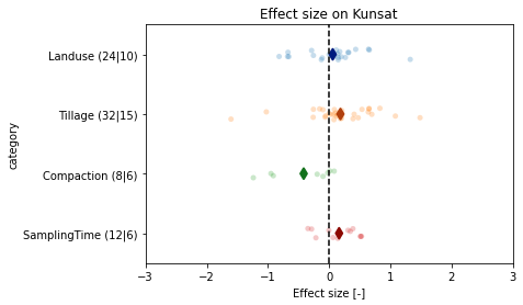
Interpretation:
- landuse +: landuse other than 'arable' have a higher K
- tillage +: tillage other than 'zero tillage' have a higher K
- crop rotation: -: crop rotation other than 'monoculture' have a lower K <=> monoculture have a higher K
- residues -: 'no residues' have higher K than when residue are left in the field (a bit uncertain)
- grazing -: 'no grazing' have a higher K than when grazed
- irrigation -: 'no irrigation' have a higher K than when irrigated
- compaction -: 'no compaction' have a higher K than when compacted
- samplingTime +: 'no impact have a lower K than after disturbance (=tillage operation)
# plot effect sizes
esColumns = ['es' + a[2][2:] for a in controls]
titles = [
    r'(a) $log_{10}\frac{\mathrm{arable}}{\mathrm{not\ arable}}$',
    r'(b) $log_{10}\frac{\mathrm{tillage}}{\mathrm{no\ tillage}}$',
    r'(c) $log_{10}\frac{\mathrm{compacted}}{\mathrm{not\ compacted}}$',
    r'(d) $log_{10}\frac{\mathrm{soon\ after\ till.}}{\mathrm{consolidated}}$']
fig, axs = plt.subplots(1, 4, figsize=(10, 3), sharex=True, sharey=False)
axs = axs.flatten()
colors = plt.rcParams['axes.prop_cycle'].by_key()['color']
for i, esColumn in enumerate(esColumns):
    ax = axs[i]
    #ax.set_title('({:s}) {:s}'.format(letters[i], esColumn[2:]))
    ax.set_title(titles[i], fontsize=14)
    ax.axvline(0, linestyle='--', color='k')
    ylabs = []
    for j, kcol in enumerate(kcols):
        col = esColumn + '_' + kcol
        #cax = ax.errorbar(dflu[col].mean(), j, xerr=dflu[col].sem(), marker='o', color=colors[i])
        df = dflu[dflu[col].notnull()]
        cax = ax.errorbar((df[col]*df['wi']).sum()/df['wi'].sum(),
                j, xerr=(df[col].std()*np.sqrt(df['wi'].pow(2).sum()))/df['wi'].sum(),
            marker='o', color=colors[i])
        # ylabs.append('{:3s}{:>9s}'.format(kcol,
        #         '({:d}|{:d})'.format(dflu[col].notnull().sum(),
        #         dflu[dflu[col].notnull()]['ReferenceTag'].unique().shape[0])))
        ylabs.append('{:3s}'.format(kcol))
    ax.set_yticks(np.arange(len(ylabs)))
    ax.set_yticklabels(ylabs, ha='right')
    if i > 3:
        ax.set_xlabel('Effect size [-]')
fig.tight_layout()
fig.savefig(outputdir + 'meta-all-k.jpg', dpi=500)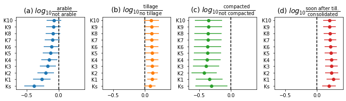
Sensitivity
Multiple methods:
- remove studies with the lowest standard deviation first Meyer et al. 2018
- remove studies with the largest weight first
- repeat for number of study (N): remove one (two, three, ...) studies and compute back the mean ES -> compute the mean and sem of the N meaned ES obtained (I think it's what Basche and deLong (2019) do)
# passing variables
escols = esColumns
escols = ['esLanduse_K10', 'esTillage_K10', 'esCompaction_K10', 'esSamplingTime_K10',
          'esLanduse_Ks', 'esTillage_Ks', 'esCompaction_Ks', 'esSamplingTime_Ks']
#escols = ['esLanduse_Ks', 'esTillage_Ks', 'esCompaction_Ks', 'esSamplingTime_Ks']
df = dflu
#variables = esColumns
#variables = ['esLanduse_Ks', 'esTillage_Ks', 'esCompaction_Ks', 'esSamplingTime_Ks']
# sensitivity of effect sizes per study (Meyer et al. 2018)
# we remove the study with the lowest standard deviation (or the largest weight) - but so we need to have the SD!
dfsens = pd.DataFrame()
for col in escols:
ie = df[col].notnull()
studySEM = df[ie].groupby('ReferenceTag').sem().reset_index().sort_values(by=col).reset_index()
#studyWeight = df[ie].groupby('ReferenceTag').sum().reset_index().sort_values(by='wi', ascending=False).reset_index()
#print(col, studySEM[col].values, studyWeight['wi'].values)
for i in range(0, 10): # number of study to exclude
studyOut = studySEM[i:]['ReferenceTag'].tolist()
#studyOut = studyWeight[i:]['ReferenceTag'].tolist()
i2keep = df['ReferenceTag'].isin(studyOut)
ie2 = ie & i2keep
nstudy = df[ie2]['ReferenceTag'].unique().shape[0]
#mean, sem = df[ie2][col].mean(), df[ie2][col].sem() # not weighted
sdf = df[ie2]
sdf = sdf[sdf[col].notnull()]
mean = (sdf[col]*sdf['wi']).sum()/sdf['wi'].sum()
sem = (sdf[col].std()*np.sqrt(sdf['wi'].pow(2).sum()))/sdf['wi'].sum()
dfsens = dfsens.append({'var': col.replace('_ES',''), 'nexcl': i, 'mean': mean,
'sem': sem, 'n': np.sum(ie2), 'nstudy': nstudy},
ignore_index=True)
dfsens.head()# sensitivity of effect sizes per study with a Jacknife technique (Basche and deLonge 2019)
dfsens = pd.DataFrame()
for col in escols:
ie = df[col].notnull()
studies = df[ie]['ReferenceTag'].unique()
sdf = df[ie]
mean = (sdf[col]*sdf['wi']).sum()/sdf['wi'].sum()
sem = 0
dfsens = dfsens.append({'var': col.replace('_ES',''), 'nexcl': 0, 'mean': mean,
'sem': sem, 'n': np.sum(ie), 'nstudy': len(studies)},
ignore_index=True)
for i in range(1, 10): # need to start at 1 with this method
means = []
sems = []
if i < len(studies):
for j in range(50):
# doing all combinations is not possible so we just take out studies
# randomly without replacement and we repeat this a number of times
studyOut = studies[np.random.choice(len(studies), size=i, replace=False)]
i2keep = ~df['ReferenceTag'].isin(studyOut)
ie2 = ie & i2keep
#mean, sem = df[ie2][col].mean(), df[ie2][col].sem() # not weighted
sdf = df[ie2]
mean = (sdf[col]*sdf['wi']).sum()/sdf['wi'].sum()
sem = (sdf[col].std()*np.sqrt(sdf['wi'].pow(2).sum()))/sdf['wi'].sum()
means.append(mean)
sems.append(sem)
mean = np.mean(means)
sem = np.mean(sem)
# sem = np.std(vals)/np.sqrt(len(vals)) # this becomes tiny as we repeat more
nstudy = len(studies) - i
dfsens = dfsens.append({'var': col.replace('_ES',''), 'nexcl': i, 'mean': mean,
'sem': sem, 'n': np.sum(ie2), 'nstudy': nstudy},
ignore_index=True)
dfsens.head()# sensitivity graphs
fig, axs = plt.subplots(2, 4, figsize=(9, 6), sharex=True, sharey=True)
axs = axs.flatten()
ts = [r'K$_{100}$', r'K$_{100}$', r'K$_{100}$', r'K$_{100}$',
r'K$_s$', r'K$_s$', r'K$_s$',r'K$_s$']
for i, variable in enumerate(escols):
ax = axs[i]
ie = dfsens['var'] == variable
ie0 = dfsens['nexcl'] == 0
ax.set_title('({:s}) {:s} ({:s})'.format(
letters[i], variable[2:].split('_')[0], ts[i]))# variable.split('_')[1]))
ax.annotate('{:.0f} refs'.format(
dfsens[ie & ie0]['nstudy'].values[0]), (0.4, 0.2))
ax.errorbar(dfsens[ie]['mean'], dfsens[ie]['nexcl'], xerr=dfsens[ie]['sem'],
marker='.', linestyle='none', color='k')
if i > 3:
ax.set_xlabel('Effect size')
if i % 4 == 0:
ax.set_ylabel('Number of studies excluded')
ax.axvline(0, color='k', linestyle=':')
ax.set_xlim([-1, 1]);
ax.invert_yaxis()
fig.tight_layout()
fig.savefig(outputdir + 'meta-sensitivity.jpg', dpi=500)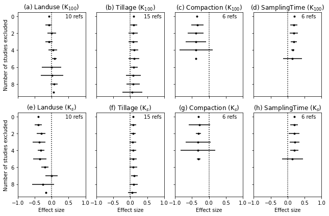
Funnel plots
# funnel plot (mean effect size vs 1/sem)
dfg = df.groupby('ReferenceTag')
dffun = dfg.mean().rename(columns=dict(zip(escols, [a + '_mean' for a in variables])))
for a in variables:
    dffun[a + '_sem'] = dfg.sem()[a]
dffun = dffun.reset_index()
dffun.head()---------------------------------------------------------------------------KeyError Traceback (most recent call last)~\WPy64-3890\python-3.8.9.amd64\lib\site-packages\pandas\core\indexes\base.py in get_loc(self, key, method, tolerance)
3079 try:
-> 3080 return self._engine.get_loc(casted_key)
3081 except KeyError as err:
pandas\_libs\index.pyx in pandas._libs.index.IndexEngine.get_loc()
pandas\_libs\index.pyx in pandas._libs.index.IndexEngine.get_loc()
pandas\_libs\hashtable_class_helper.pxi in pandas._libs.hashtable.PyObjectHashTable.get_item()
pandas\_libs\hashtable_class_helper.pxi in pandas._libs.hashtable.PyObjectHashTable.get_item()
KeyError: 'esLanduse'
The above exception was the direct cause of the following exception:
KeyError Traceback (most recent call last)<ipython-input-102-f89cebe36919> in <module>
3 dffun = dfg.mean().rename(columns=dict(zip(escols, [a + '_mean' for a in variables])))
4 for a in variables:
----> 5 dffun[a + '_sem'] = dfg.sem()[a]
6 dffun = dffun.reset_index()
7 dffun.head()
~\WPy64-3890\python-3.8.9.amd64\lib\site-packages\pandas\core\frame.py in __getitem__(self, key)
3022 if self.columns.nlevels > 1:
3023 return self._getitem_multilevel(key)
-> 3024 indexer = self.columns.get_loc(key)
3025 if is_integer(indexer):
3026 indexer = [indexer]
~\WPy64-3890\python-3.8.9.amd64\lib\site-packages\pandas\core\indexes\base.py in get_loc(self, key, method, tolerance)
3080 return self._engine.get_loc(casted_key)
3081 except KeyError as err:
-> 3082 raise KeyError(key) from err
3083
3084 if tolerance is not None:
KeyError: 'esLanduse'fig, axs = plt.subplots(2, 4, figsize=(8,6), sharex=True, sharey=True)
axs = axs.flatten()
for i, a in enumerate(variables):
ax = axs[i]
inan = dffun[a + '_mean'].isna()
ax.set_title('{:s} (n={:.0f})'.format(a[2:], dffun[~inan]['ReferenceTag'].unique().shape[0]))
ax.axvline(dffun[a + '_mean'].mean(), color='k', linestyle='--')
ax.plot(dffun[a + '_mean'], 1/dffun[a + '_sem'], 'b.')
if i % 4 == 0:
ax.set_ylabel('Inverse of standard deviation')
if i > 3:
ax.set_xlabel('Mean effect size')
fig.tight_layout()
fig.savefig(outputdir + 'meta-funnel.jpg', dpi=500)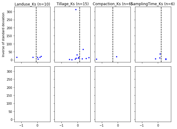
# another approach is to just plot the histogram of effect sizes (Bashe and deLonge 2017)
fig, axs = plt.subplots(1, 4, figsize=(8, 3), sharex=True, sharey=True)
axs = axs.flatten()
bins = np.linspace(-2, 2, 11)
for i, esColumn in enumerate(esColumns):
    ax = axs[i]
    ax.set_title('({:s}) '.format(letters[i]) + esColumn[2:])
    ax.hist(dflu[esColumn].dropna().values, bins=bins)
    ax.axvline(0, color='k', linestyle='--')
    if i >= 4:
        ax.set_xlabel('Effect size [-]')
    if i % 4 == 0:
        ax.set_ylabel('Number of ES')
fig.tight_layout()
fig.savefig(outputdir + 'hist-es.jpg', dpi=500)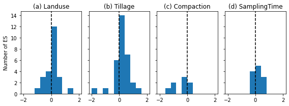
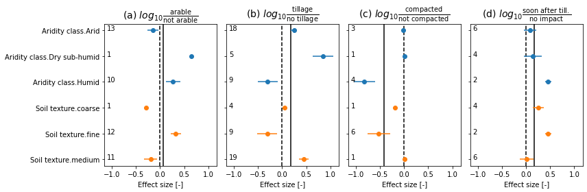
Heterogeneity
How much effect size varies according to different sub categories.
smth like in young

so using other columns to dissect the ES in subgroups of interest (after/before disturbance for instance) or by soil type
# TODO disc size, soil texture fao, sampling time, soc classes, aridity class, with/without cover crops

# create classes
dflu['Aridity class'] = dflu['AridityClass'].replace({'Hyper Arid': 'Arid', 'Semi-Arid': 'Arid'})
dflu['Annual precipitation'] = pd.cut(dflu['AnnualPrecipitation'], bins=[0, 200, 400, 600, 2000])
dflu['Annual mean temperature'] = pd.cut(dflu['AnnualMeanTemperature'], bins=[0, 10, 15, 30])
gcol = 'SoilTextureUSDA'
def func(x):
    dico = {
        'unknown': np.nan,
        np.nan: np.nan,
        'organic': np.nan,
        'clay': 'fine',
        'clay loam': 'fine',
        'loam': 'medium',
        'loamy sand': 'coarse',
        'sand': 'coarse',
        'sandy clay': 'coarse',
        'sandy clay loam': 'coarse',
        'sandy loam': 'coarse',
        'silt loam': 'medium',
        'silty clay': 'fine',
        'silty clay loam': 'fine'
    }
    return dico[x]
dflu['Soil texture'] = dflu['SoilTextureUSDA'].apply(func)
dflu['Soil organic carbon'] = pd.cut(dflu['SoilOrganicCarbon'], bins=[0.0, 0.01, 0.02, 0.03, 0.1])


# figure
#colgroup = ['Aridity class', 'Annual precipitation', 'Annual mean temperature', 'Soil texture', 'Soil organic carbon']
colgroup = ['Aridity class', 'Soil texture']
titles = [
    r'(a) $log_{10}\frac{\mathrm{arable}}{\mathrm{not\ arable}}$',
    r'(b) $log_{10}\frac{\mathrm{tillage}}{\mathrm{no\ tillage}}$',
    r'(c) $log_{10}\frac{\mathrm{compacted}}{\mathrm{not\ compacted}}$',
    r'(d) $log_{10}\frac{\mathrm{soon\ after\ till.}}{\mathrm{no\ impact}}$']
fig, axs = plt.subplots(1, len(esColumns), sharex=True, sharey=True, figsize=(12, 4))
axs = axs.flatten()
for i, esColumn in enumerate(esColumns):
    ax = axs[i]
    # ax.set_title('({:s})\n'.format(letters[i]) + esColumn[2:] +
    #             '\n({:d}|{:d})'.format(dflu[esColumn].notnull().sum(),
    #             dflu[dflu[esColumn].notnull()]['ReferenceTag'].unique().shape[0]))
    ax.set_title(titles[i], fontsize=14)
    y = 0
    ylabs = []
    ax.axvline(0, linestyle='--', color='k')
    ax.axvline(dflu[esColumn].mean(), color='k')
    for col in colgroup:
        dfg = dflu.groupby(col)
        color = None
        for key, group in dfg:
            if (group[esColumn].notnull().sum() > 0) and (key != 'unknown'):
                cax = ax.errorbar(group.mean()[esColumn],
                                  xerr=group.sem()[esColumn],
                                  y=y, marker='o', color=color)
                ax.text(-1.1, y, str(group[esColumn].notnull().sum()))
                if color is None:
                    color = cax[0].get_color()
                y += 1
                ylabs.append(col + '.' + str(key))# + ' ({:d})'.format(group[esColumn].dropna().shape[0]))
    ax.set_xlabel('Effect size [-]')
    if i == 0:
        ax.set_yticks(np.arange(len(ylabs)))
        ax.set_yticklabels(ylabs)
        ax.invert_yaxis()
fig.tight_layout()
fig.savefig(outputdir + 'split-es.jpg', dpi=500)
/tmp/ipykernel_68428/840661095.py:55: FutureWarning: Dropping of nuisance columns in DataFrame reductions (with 'numeric_only=None') is deprecated; in a future version this will raise TypeError. Select only valid columns before calling the reduction.
cax = ax.errorbar(group.mean()[esColumn],
/tmp/ipykernel_68428/840661095.py:56: FutureWarning: Dropping of nuisance columns in DataFrame reductions (with 'numeric_only=None') is deprecated; in a future version this will raise TypeError. Select only valid columns before calling the reduction.
xerr=group.sem()[esColumn],
# meta-regression are more adapted for continuous variable
hcols = {
    'AverageAridityIndex': ['Average aritidy index [-]', None, None],
    #'AnnualPrecipitation': ['Mean annual precipitation [mm]', 0, 2000],
    'AnnualMeanTemperature': ['Annual mean temperature [degC]', 0, 35],
    'SoilOrganicCarbon': ['Soil organic carbon [gC/kg]', 0, 0.03],
    'MeanDiurnalRange': ['Diurnal range [degC]', None, None]
}
kcols = ['Ks']
practices = {
    'Landuse': 'Land use',
    'Tillage': 'Tillage',
    'Compaction': 'Compaction',
    'SamplingTime': 'Sampling time'
}

fig, axs = plt.subplots(len(practices), len(hcols), sharey=True, figsize=(12, 8))
for i, prac in enumerate(practices):
    for j, xcol in enumerate(hcols):
        ylab = practices[prac]
        ax = axs[i, j]
        ax.axhline(0, linestyle='--', color='k')
        ax.annotate(letters[i*len(practices)+j], (0.05, 0.85), xycoords='axes fraction', fontsize=14)
        for kcol in kcols:
            ycol = 'es' + prac + '_' + kcol
#            ax.plot(dflu[xcol], dflu[ycol], 'o', label=kcol)
            sns.regplot(x=dflu[xcol], y=dflu[ycol], label=kcol, ax=ax)
        if j == 0:
            ax.set_ylabel(ylab + ' ES')
        else:
            ax.set_ylabel('')
        ax.set_xlim(hcols[xcol][1:])
        if i == len(hcols) - 1:
            ax.set_xlabel(hcols[xcol][0])
        else:
            ax.set_xlabel('')
        if i == 0 and j == 0:
            ax.legend()
fig.tight_layout()
fig.savefig(outputdir + 'meta-regression-ks.jpg', dpi=500)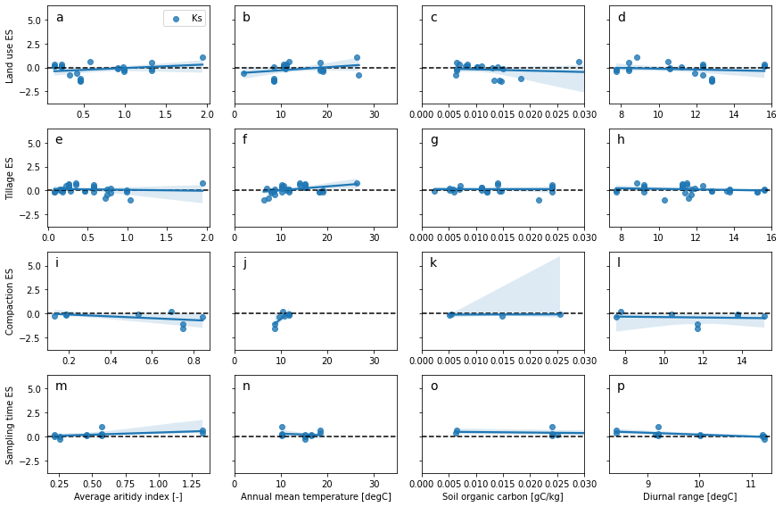
# meta-regression are more adapted for continuous variable
hcols = {
    'AverageAridityIndex': ['Average aritidy index [-]', None, None],
    #'AnnualPrecipitation': ['Mean annual precipitation [mm]', 0, 2000],
    'AnnualMeanTemperature': ['Annual mean temperature [degC]', 0, 35],
    'SoilOrganicCarbon': ['Soil organic carbon [gC/kg]', 0, 0.03],
    'MeanDiurnalRange': ['Diurnal range [degC]', None, None]
}
kcols = ['K10']
practices = {
    'Landuse': 'Land use',
    'Tillage': 'Tillage',
    'Compaction': 'Compaction',
    'SamplingTime': 'Sampling time'
}

fig, axs = plt.subplots(len(practices), len(hcols), sharey=True, figsize=(12, 8))
for i, prac in enumerate(practices):
    for j, xcol in enumerate(hcols):
        ylab = practices[prac]
        ax = axs[i, j]
        ax.axhline(0, linestyle='--', color='k')
        ax.annotate(letters[i*len(practices)+j], (0.05, 0.85), xycoords='axes fraction', fontsize=14)
        for kcol in kcols:
            ycol = 'es' + prac + '_' + kcol
#            ax.plot(dflu[xcol], dflu[ycol], 'o', label=kcol)
            sns.regplot(x=dflu[xcol], y=dflu[ycol], label=kcol, ax=ax)
        if j == 0:
            ax.set_ylabel(ylab + ' ES')
        else:
            ax.set_ylabel('')
        ax.set_xlim(hcols[xcol][1:])
        if i == len(hcols) - 1:
            ax.set_xlabel(hcols[xcol][0])
        else:
            ax.set_xlabel('')
        if i == 0 and j == 0:
            ax.legend()
fig.tight_layout()
fig.savefig(outputdir + 'meta-regression-k10.jpg', dpi=500)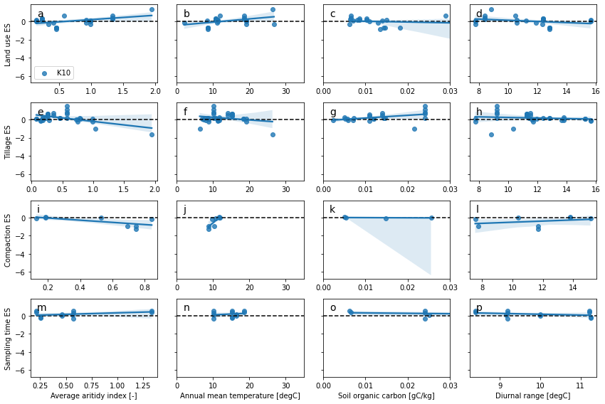
# figure of pure interactions
dflu['NbOfCropRotationStr'] = dflu['NbOfCropRotation'].astype(str)
colgroup = ['LanduseClass', 'TillageClass', 'ResidueClass',
            'GrazingClass', 'IrrigationClass', 'CompactionClass', 'SamplingTimeClass']
fig, axs = plt.subplots(1, len(esColumns), sharex=True, sharey=True, figsize=(14, 5))
axs = axs.flatten()
plt.text(0.02, 0.9, 'K10', fontsize=14, transform=plt.gcf().transFigure)
for i, esColumn in enumerate(esColumns):
    ax = axs[i]
    ax.set_title('({:s})\n'.format(letters[i]) + esColumn[2:] +
                '\n({:d}|{:d})'.format(dflu[esColumn].notnull().sum(),
                dflu[dflu[esColumn].notnull()]['ReferenceTag'].unique().shape[0]))
    y = 0
    ylabs = []
    ax.axvline(0, linestyle='--', color='k')
    #ax.errorbar(dflu[esColumn].mean(), 0, xerr=dflu[esColumn].sem(), color='k', marker='o')
    ax.axvline(dflu[esColumn].mean(), color='k')
    #ylabs.append('Grand mean')
    for col in colgroup:
        dfg = dflu.groupby(col)
        color = None
        ax.axhline(y-0.5, linestyle=':', color='lightgrey')
        for key, group in dfg:
            if (group.shape[0] > 3) and (key != 'unknown'):
                cax = ax.errorbar(group.mean()[esColumn],
                                  xerr=group.sem()[esColumn],
                                  y=y, marker='o', color=color)
                if color is None:
                    color = cax[0].get_color()
                y += 1
                #ylabs.append('{:*<15s} {:*>15s}'.format(col.replace('Class', ''), key))
                ylab = '{:s}.{:s}'.format(col.replace('Class', ''), key)
                for row in controls:
                    if row[0] == col and row[1] == key:
                        ylab = '*' + ylab
                        break
                ylabs.append(ylab)
    ax.set_xlabel('Effect size [-]')
    if i == 0:
        ax.set_yticks(np.arange(len(ylabs)))
        ax.set_yticklabels(ylabs)
        ax.invert_yaxis()
#fig.tight_layout()
fig.subplots_adjust(left=0.17)
fig.savefig(outputdir + 'split-es-col.jpg', dpi=500)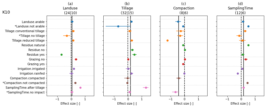
- Meyer, N., Bergez, J.-E., Constantin, J., & Justes, E. (2018). Cover crops reduce water drainage in temperate climates: A meta-analysis. Agronomy for Sustainable Development, 39(1). 10.1007/s13593-018-0546-y
- Basche, A. D., & DeLonge, M. S. (2019). Comparing infiltration rates in soils managed with conventional and alternative farming methods: A meta-analysis. PLOS ONE, 14(9), e0215702. 10.1371/journal.pone.0215702