Quantitative meta-analysis, publication bias and machine-learning to derive context-specific relationships
Summary
Saturated and near-saturated soil hydraulic conductivities Kh (mm.h-1) determine the partitioning of precipitation into surface runoff and infiltration. They are fundamental to soils’ susceptibility to preferential flow and indicate soil aeration properties. However, measurements of saturated and near-saturated soil hydraulic conductivities are time consuming. So-called pedotransfer functions are needed to estimate Kh from predictor variables. Since respective pedotransfer functions have been largely unsuccessful, recent studies have focused on assembling and analysing bigger databases, aiming at finding better predictors. In this work package, we collated OTIM-DB (Open Tension-disk Infiltrometer Meta-database), which builds on a meta-database published by Jarvis, N., Koestel, J., Messing, I., Moeys, J., and Lindahl, A.: Influence of soil, land use and climatic factors on the hydraulic conductivity of soil, Hydrol. Earth Syst. Sci., 17, 5185–5195, 2013. OTIM-DB increases the number of data-entries by a factor of approximately 1.5 compared to its predecessor and contains more detailed information on local climate as well as land use and management than its predecessor. In this study, we present OTIM-DB together with a meta-analysis on topsoil Kh from supply tensions ranging between 0 and 10 cm. We also included an attempt to build a respective pedotransfer function using a light gradient boosting model.
Our study confirmed significant correlations between climate variables as well as the elevation above sea level with Kh. While it seems very likely that these variables influence soil physical properties, the exact underlying mechanisms need to be investigated in future studies. We found indications that specific soil management practises lead to changes in Kh. They were increased under perennial cultures and decreased for no-till arable fields with annual crops and for compacted soil. Our data also confirmed that it is fundamental to take the time of the measurement after the last tillage operation into account to understand relationships between soil management and Kh. Note that the management impacts turned out to be dependent on the pedo-climatic context, as they only could be observed if variations in the latter were ruled out. Besides these results, we also found that the data availability for tension-disk infiltrometer data was too scarce and riddled with too many gaps for detailed analyses of other soil management impacts, more specific pedo-climatic context dependencies and publication bias. Furthermore, we found evidence that the available data was afflicted with experimenter bias. Altogether, it was not possible to predict Kh from the available data for new sites, which echoes results of similar attempts to build respective pedotransfer functions. More measurements with better documented meta-data and better suited predictor variables would be needed for progress in this field. Studies quantifying soil structure evolution with respect to season, land use and soil management using X-ray imaging may turn out to provide useful information for more appropriate predictor variables for Kh.
Introduction
Soil climate models predict more frequent extreme events with the onset of global warming such as high intensity rainfall. To prevent water runoff and erosion on fields, the soils need to be able to conduct such large amounts of water in a short time. The soil property that matters is the saturated hydraulic conductivity Ks (mm.h-1). It determines the partitioning of precipitation into surface runoff and infiltration. A large Ks reduces erosion risks and allows water to infiltrate into deeper soil layers, where it may replenish an important reservoir of plant available water or contribute to groundwater recharge. The hydraulic conductivity of a soil decreases with decreasing water content, i.e. with decreasing water saturation. The hydraulic conductivity in this so-called near-saturated range is likewise important. Soils with larger hydraulic conductivity near saturation Kh (mm.h-1) tend to generate less water flow in macropore networks. Therefore, they are less susceptible to preferential flow Larsbo , 2014 by which agrochemicals and other solutes quickly leach towards the groundwater. Moreover, large Kh also indicates a well-aerated soil, which drains faster and helps air to escape the soil in cases of heavy rainfall. This further reduces the risk of surface runoff and erosion as entrapped air strongly decreases soil hydraulic conductivity. Note that the index ‘h’ indicates a matrix potential between 0 and 10 cm at which Kh was measured. References to Kh may also include Ks since for h == 0 cm, Kh == Ks.
Saturated hydraulic conductivity is measured either in the laboratory on small cylinders, usually with diameters < 7 cm Klute & Dirksen, 1986 or it is acquired from field measurements, either using single or double ring methods Angulo-Jaramillo , 2000. In addition, the near-saturated hydraulic conductivities can be measured using a tension disk infiltrometer. The method is designed as a field method but has been occasionally applied in the lab. Using a tension disk hydraulic conductivities between ca. 0.5 and ca. 60 to 150 mm can be obtained, depending on the specifications of the infiltrometer. All measurement techniques for the saturated and near-saturated hydraulic conductivities are laborious, time-consuming and constrained to a relatively small soil volume.
It is therefore necessary to develop pedotransfer functions to estimate soil hydraulic conductivities for modelling applications Bouma, 1989Van Looy , 2017Wösten , 2001. The development of a pedotransfer function requires a database from which it can be derived. For example, the well-known pedotransfer function ROSETTA Schaap , 2001 is based on the open UNSODA database Nemes , 2001. The equations published in Tóth (2015) are derived from the proprietary EU-HYDI database Weynants , 2013. The pedotransfer functions of Jarvis (2013) are based on an unpublished meta-database containing tension-disk infiltrometer data.
Collecting published measurements of saturated and near-saturated hydraulic conductivity measurements into meta-databases and pairing them with other existing databases is essential to develop pedotransfer functions. A notable example is the SWIG database Rahmati , 2018 that collates more than 5000 datasets from soil infiltration measurements, covering the entire globe. Another big effort in collecting information on saturated hydraulic conductivity is the newly published SoilKsatDB Gupta , 2021, which combines saturated hydraulic conductivity data from several large databases, amongst others UNSODA and SWIG, together with additional measurements published in independent scientific studies. However, none of the databases cited above provide open-access infiltration measurements at tension near-saturation (h > 0 mm), which limits their use to estimations of saturated hydraulic conductivities.
Pedotransfer functions for saturated hydraulic conductivity exhibit rather poor predictive performance Weynants , 2009Jorda , 2015 . Early approaches, like HYPRES Wösten , 1999 and ROSETTA, focused solely on soil properties like texture, bulk density and organic carbon content. Back then, it was not sufficiently recognized that soil Ks is mostly determined by the morphology of macropore networks, especially in finer-textured soils Vereecken , 2010Koestel , 2018Schlüter , 2020. A pedotransfer function for Ks requires therefore ideally a database that contains direct information on the macropore network itself. But since such measures are more cumbersome and time-consuming to obtain (e.g. by X-ray tomography) than measuring hydraulic conductivity itself, it is more reasonable and makes more sense to use proxies from which the macrostructure in a soil can be inferred. Ideal candidates would be root growth and the activity of soil macrofauna, which both strongly determine the development of macropore networks in soil Meurer (2020). But also they are difficult to measure. More promising proxies are land use and farming practises, such as tillage or soil compaction due to trafficking. Plant growth and soil macrofauna are in turn influenced by the local climate. The climate also sets boundaries for the land use and the associated soil management practises, and thus provides feedback to root growth and macro-faunal activity. Wetting and drying cycles, and thus the formation and closure of cracks also are regulated by the climate. It is therefore not surprising that climate variables are typically correlated with saturated and near-saturated hydraulic conductivities Jarvis , 2013Jorda , 2015Hirmas , 2018Gupta , 2021. Jorda (2015) found that land use itself was the most important predictor for saturated hydraulic conductivity. The time of measurement of the hydraulic conductivity (or soil sampling) also has a crucial impact. In an agricultural soil, the hydraulic properties of a freshly prepared seedbed differ from those measured later at harvest. Several studies have demonstrated the evolution of hydraulic conductivity with time Messing & Jarvis, 1990Bodner , 2013Sandin , 2017 . Soil management options (such as tillage or the use of cover crops) actively influence the soil saturated and near-saturated hydraulic conductivity. Information on their impact is therefore especially important, but so far has hardly been investigated in meta-analyses.
Quantitative analyses of meta-databases are referred to as meta-analyses. It often consists either of an exploratory data analysis or a comparison of effect sizes or both. The the second method compares effects of two different treatments, i.e. conventional and reduced tillage, on the target variables, in our case Kh. Individual source publications need to contain results for both treatments. The observed differences in each study are then averaged and interpreted. An example of such a study is Basche & DeLonge (2019). For the exploratory data analysis, data entries from the meta-database are evaluated using weighted correlations, regressions or cluster analyses. The weighting is important, because the source publications provide different amounts of data entries to the meta-database that are in turn summarised from varying numbers of replications. Data entries measured at the same field site need to be down-weighted, as they would otherwise introduce a bias that would make the respective site properties, e.g. the climate at this site, appear disproportionately important. Likewise, data entries that represent the average of several replications need to be up-weighted compared to data entries representing the average of only a single measurement.
Relationships between environmental data are often non-linear. In such cases, predictions made linear regressions contain considerable error due to under-fitting, i.e. introduced by using a linear model to express a non-linear relationship. Modern machine learning approaches have the advantage that they can model non-linear relationships. They also enable quantifications of predictor importance and their comparison, offering a way to compare categorical with numerical predictors. By singling out the most important predictors, context-specific relationships in dependence of these predictors can be evaluated, provided that the investigated dataset is large enough.
In this study, we investigated the effects of soil management practises on the saturated and near-saturated hydraulic conductivity, including analyses of publication bias. More specifically, we illustrated the statistical relationships between soil properties and pedo-climatic and agronomic factors and saturated and near-saturated hydraulic conductivity in the tension range from 0 to 10 cm. To our knowledge, a systematic and quantitative review on hydraulic conductivity over the entire near-saturated tension range has been missing in peer-reviewed literature. Through this work, we expanded and published the previously unpublished meta-database on tension-disk infiltration measurements that was first reported by Jarvis (2013). We referred to this database as OTIM-DB in the following (Open Tension-disk Infiltrometer Meta-Database). It complements the currently available public databases that are strongly based on laboratory measurements or ring infiltrometer methods. OTIM-DB allows the investigation of systematic bias in saturated hydraulic conductivity measurements due to the method applied and supports the development of improved pedotransfer functions for saturated and near-saturated hydraulic conductivities.
In the first part of the report of CLIMASOMA WP4, we present OTIM-DB and undertake meta-analyses (TP1) and attempt to appraise publication bias in the included source-publications (TP2). In the second part, we discuss the result of a machine learning approach trained on the OTIM-DB data (TP3).
Meta-Database, OTIM-DB
Data collection
The first version of OTIM-DB was compiled for the study by Jarvis (2013). The original database contained 753 tension-disk infiltrometer data entries collated from 124 source publications, covering 144 different locations around the globe. We have extended this database by 577 new tension-disk infiltrometer data entries from 48 additional studies that had been published after 2012. The search for publications was carried out between 2021-05-31 and 2021-06-23 using the queries and search engines detailed in Table S1.
We found 115 publications containing tension-disk infiltrometer measurements published in 2013 or later. We retained the data for further analysis when (i) Kh or the infiltration rate was measured at more than two tensions larger or equal 5 mm and (ii) sufficient meta-data on soil and site properties (at least soil texture) as well as soil management practises (at least land use and tillage) were available. When a publication solely reported infiltration rates, we calculated the hydraulic conductivity using the method of Ankeny (1991). Only 45 of the 115 publications fulfilled the above-mentioned criteria. Table S2 summarises how many papers were rejected for which reasons. For 27 of the 45 retained studies, we digitised the published Kh values from figures using WebPlotDigitizer (open-source web-based software created by Ankit Rohatgi, https://automeris.io/WebPlotDigitizer/). For cases in which Kh measurements were mentioned in a publication, but the results were not reported, we contacted the corresponding authors. For three of these publications, we received the data in this fashion Alletto , 2015Larsbo , 2016Meshgi & Chui, 2014.
In addition to adding data from new publications to OTIM-DB, we also revisited the studies already contained in the original database version and collected additional information on soil management practises associated with the measured data. For each soil management option, OTIM-DB contains two columns. In the first column, the information as given in the source publication is stored. The second column summarises this information into a few classes, which could subsequently be used in the meta-analysis. In this study, we investigated effects of land use, tillage system, soil compaction and day of measurement relative to the latest tillage operation on the field. A compaction class was assigned to a data entry only if the plot had been described as ‘compacted’ or ‘not compacted’ in the source publication. ‘Compacted’ data entries corresponded, for example, to infiltration measurements in wheel tracks or on plots of a compaction experiment. The day of measurement was labelled ‘after tillage’ when the authors in the source publication stated that the measurements had taken place within a few weeks after tillage. Otherwise, it was assumed that the soil had already had time to consolidate before the infiltration measurement was carried out. All soil texture data was mapped onto the USDA classification using the method proposed in Nemes (2001).
List of new entries added to theJarvis (2013) database.
Reference | Land use | Tillage | Compaction | Sampling time | Data entries |
|---|---|---|---|---|---|
grassland | no tillage | not compacted | consolidated soil | 1 | |
arable | conventional tillage | unknown | consolidated soil | 60 | |
arable | no tillage | conventional tillage | unknown | unknown | 10 | |
grassland | arable | no tillage | not compacted | compacted | unknown | consolidated soil | 4 | |
arable | reduced tillage | no tillage | conventional tillage | unknown | consolidated soil | soon after tillage | 12 | |
arable | no tillage | unknown | soon after tillage | consolidated soil | 12 | |
arable | unknown | conventional tillage | reduced tillage | no tillage | unknown | consolidated soil | 10 | |
arable | conventional tillage | reduced tillage | no tillage | not compacted | consolidated soil | 3 | |
grassland | no tillage | not compacted | unknown | 6 | |
arable | conventional tillage | not compacted | compacted | consolidated soil | 2 | |
arable | no tillage | reduced tillage | conventional tillage | compacted | not compacted | unknown | 8 | |
arable | woodland/plantation | grassland | conventional tillage | no tillage | not compacted | compacted | unknown | 3 | |
Greenwood (2017) | arable | grassland | conventional tillage | no tillage | unknown | consolidated soil | 4 |
arable | conventional tillage | not compacted | unknown | 60 | |
arable | no tillage | not compacted | consolidated soil | 2 | |
grassland | no tillage | not compacted | consolidated soil | 5 | |
arable | conventional tillage | unknown | consolidated soil | 4 | |
arable | grassland | woodland/orchard | reduced tillage | no tillage | unknown | consolidated soil | 3 | |
arable | grassland | reduced tillage | no tillage | conventional tillage | not compacted | consolidated soil | 4 | |
arable | no tillage | conventional tillage | unknown | consolidated soil | 15 | |
arable | no tillage | unknown | unknown | 4 | |
arable | conventional tillage | not compacted | compacted | consolidated soil | unknown | 5 | |
woodland/orchard | grassland | no tillage | not compacted | consolidated soil | 4 | |
arable | no tillage | not compacted | consolidated soil | 2 | |
Lozano-Baez (2020) | grassland | woodland/orchard | no tillage | not compacted | unknown | 18 |
grassland | no tillage | unknown | unknown | 3 | |
arable | conventional tillage | unknown | consolidated soil | 10 | |
arable | conventional tillage | reduced tillage | no tillage | unknown | consolidated soil | 12 | |
arable | grassland | conventional tillage | no tillage | unknown | unknown | 4 | |
arable | conventional tillage | unknown | consolidated soil | 69 | |
arable | conventional tillage | not compacted | unknown | consolidated soil | 18 | |
arable | conventional tillage | not compacted | compacted | consolidated soil | unknown | 7 | |
grassland | conventional tillage | not compacted | compacted | unknown | 3 | |
arable | conventional tillage | no tillage | unknown | consolidated soil | 6 | |
Wang (2022) | arable | conventional tillage | unknown | soon after tillage | consolidated soil | 25 |
arable | conventional tillage | unknown | consolidated soil | 6 | |
grassland | no tillage | unknown | unknown | 11 | |
Yusuf (2018) | arable | no tillage | not compacted | consolidated soil | 1 |
arable | no tillage | not compacted | consolidated soil | 5 | |
woodland/orchard | conventional tillage | unknown | consolidated soil | 20 | |
grassland | no tillage | unknown | consolidated soil | 6 | |
grassland | arable | no tillage | unknown | unknown | consolidated soil | 6 | |
arable | conventional tillage | unknown | consolidated soil | 4 | |
woodland/orchard | arable | no tillage | conventional tillage | unknown | not compacted | consolidated soil | soon after tillage | 24 | |
grassland | woodland/orchard | arable | no tillage | conventional tillage | unknown | consolidated soil | 4 | |
arable | grassland | conventional tillage | no tillage | not compacted | unknown | 12 | |
arable | grassland | woodland/orchard | conventional tillage | no tillage | not compacted | soon after tillage | 3 |
Climate data and soil classification
The climatic data entries provided in the database were created using the bioclimatic raster data (BioClim) provided by WorldClim (worldclim.org). The data was averaged across the years 1970 to 2000 and had a 30 arc second resolution (~1 km2; Fick & Hijmans (2017)). The available climate variables were mean annual temperature and precipitation, the mean temperature as well as mean precipitation of the warmest, coldest, wettest and driest quarter and month, respectively, the isothermality, the mean diurnal and annual temperature range, the seasonality for temperature and precipitation. Besides the bio-climatic data in WorldClim we included the aridity index as well as the average annual potential evapotranspiration (ET0). Both were inferred from the “Global Aridity Index and Potential Evapotranspiration Climate Database v2” that is based on the WorldClim database Trabucco & Zomer (2019). The World Reference Base (WRB) soil type was also extracted from the source publications. When it was not reported, the SoilGrids database by ISRIC Sousa , 2020 was used to infer it. The map contained information about the main soil type regarding the WRB classes (IUSS Working Group WRB, 2015). The most probable soil type was chosen for each location. For all discussed climate and soil maps, the python package “rasterio” (v1.2.10) was used to collect the variables from the corresponding raster cell at the location coordinates given in the source publications.
Model fit to infer to Kh at near-saturated tensions not measured
Tension-disk infiltrometers measure infiltration rates at a specific supply tension Angulo-Jaramillo , 2000 that are then commonly converted to hydraulic conductivities with the aid of the Wooding equation Wooding, 1968. Note that tension-disk infiltrometers cannot provide measurements at a tension of zero, i.e. Ks. Albeit many publications report Ks values obtained from tension-disk infiltrometers, these measurements must have been conducted at tensions slightly larger than zero, as otherwise water will freely leak out of the tension disk. For this reason, we set the tensions for Ks measurements to 1 mm, but will still refer to these data as saturated hydraulic conductivity. Following Jarvis (2013), we interpolated Kh for tensions in-between the ones measured in the source publications. We achieved this by fitting a log-log linear model with a kink at a tension hmin, which denotes the tension at which the largest effective pores in the soil are water-filled (see Figure 1). Therefore, Kh == Ks for all tensions h ≤ hmin.
If Ks was not measured but instead a Kh value at h ≤ 5 mm was available, Ks was set to the available Kh value (Figure 1 orange line). In cases where more than one Kh value was measured at a tension smaller or equal to 5 mm (including h = 0 mm, i.e. Ks), we averaged them and set Ks and Kh for h ≤ hmin to the average (Figure 1 green line). Kh values at h > 5 mm were used to fit the log-log linear relationship. The tension at which the fitted log-log slope intersected with Ks defined hmin. We used the fitted model to estimate all Kh values for tensions for 10 ≤ h ≤ 100 mm at 10 mm intervals. The Kh values were only interpolated between the tensions that were measured in the source publication. The only exceptions from this rule were made in the case where a K value for a tension of 80 or 90 mm was provided together with at least one other K value measured at a smaller tension. Then, the missing K values were extrapolated up to a tension of 100 mm. Figure 1 shows examples of model fits. Only entries with an R2 greater or equal to 0.9 are retained in the analysis.
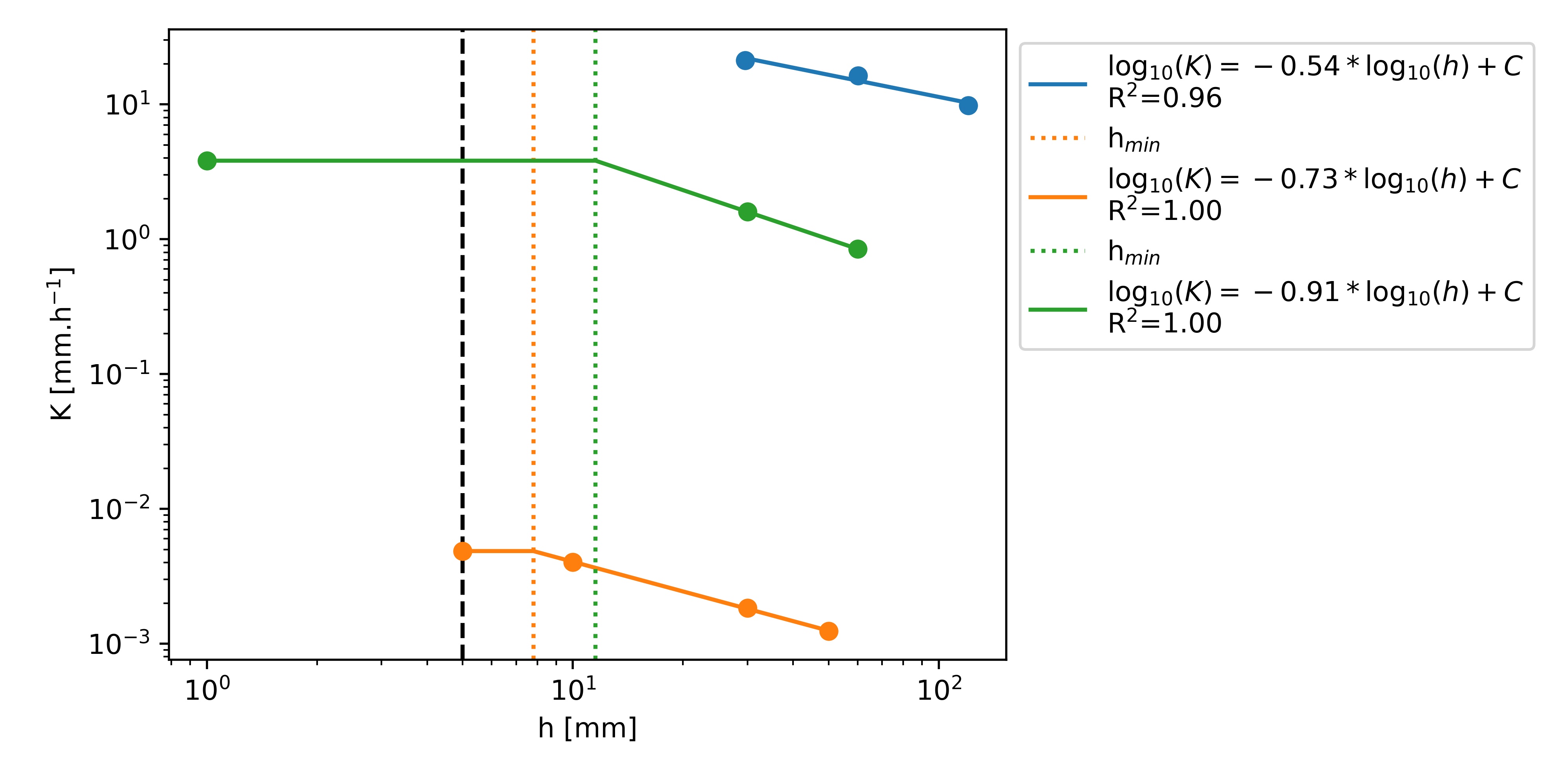
Example of linear fit in log-space. Ks values were assigned a tension of 1 mm for illustration purposes. The equations for the linear part of the fit are shown in the legend. C represents the intercept with the y-axis of the linear fit in log-space.
Database organisation
OTIM-DB is organised in 9 individual tables illustrated in Figure 2. The main table is named experiments. It contains identifiers with which all the other tables are linked. The identifiers are shown in bold font in Figure 2. The reference table contains information on the references for each study. The location table lists the coordinates of the measurement sites. The tables soilProperties, soilManagement and climate store data as implied by their names. The method table gives details on the specifications of the tension-disk infiltrometer and the method to calculate hydraulic conductivity from the infiltration rate. The rawData table contains the hydraulic conductivities and respective supply tensions as stated in the corresponding source publication. Note that OTIM-DB does not contain raw data for the entries of the original version compiled for Jarvis (2013). Finally, modelFit reports Kh for 0 ≤ h ≤ 100 mm as described above. For more details, the reader is directed to the ‘description’ tab of the database (not shown in Figure 2) where the meanings and units of each column are explained.
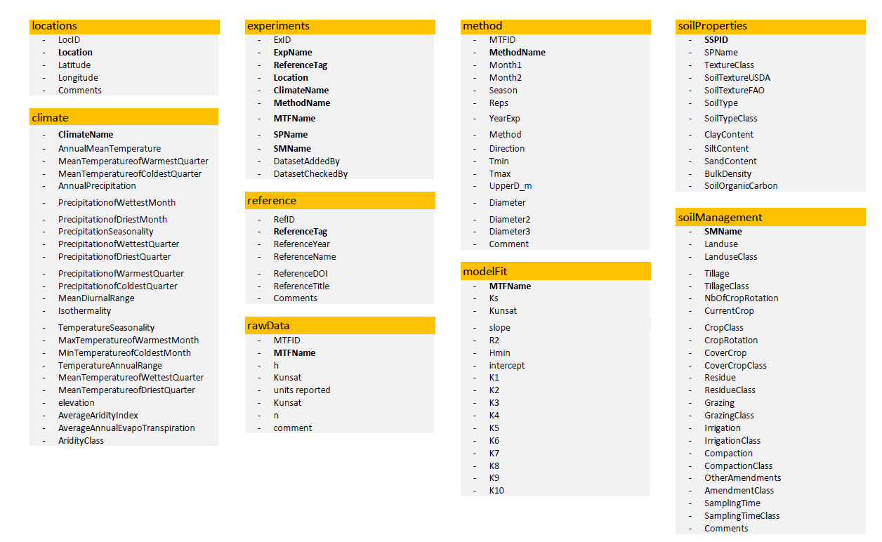
Structure of the OTIM-DB database with its different tables and columns. In the soilManagement table, the columns with the suffix “Class” denote columns in which the data reported in the source publications were summarised into classes to facilitate comparing them. For example, the reported CurrentCrop like wheat, rye, barley or oat was assigned the CropClass cereals. The rows in bold denote unique identifiers with which the table entries are linked to the experiments table.
Data availability and coverage
Although 92% of the data in OTIM-DB was obtained from measurements on the topsoil, it also contains some data points measured at greater soil depths. In the following meta-analysis, only measurements from the topsoil were included and all datasets measured at soil depths below 300 mm were removed. Also, all data entries were discarded for which the log-log linear model could not be fitted with a coefficient of determination of 0.9 or better. Last but not least, we found that the relationship between supply tension and Kh was distorted if data entries were included that did not cover the complete tension range from h = 0 to 100 mm. Possible reasons for the difficulties to match Kh data from tension series with different lengths are discussed at the beginning of the results and discussion section. Except for this discussion, we focused on data entries that included Kh values for the complete tension range in the exploratory data analysis and the meta-analyses. The available datasets after these filtering steps correspond to the ones indicated in blue (‘focus’) in the following figures.
Figure 3 shows the number of publications included in the OTIM-DB per publication year. On average, 6.7 new publications per year were published after 2000.
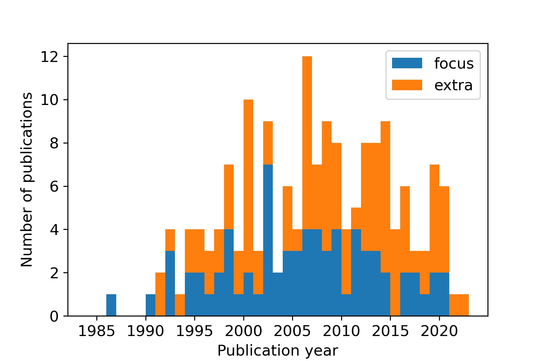
Distribution of the publication year in the OTIM-DB. Publications labelled as 'focus' contain Kh for all tensions between h = 0 and 100 mm, were measured at soil depths of less than 20 mm and exhibited coefficients of determination for the log-log linear model fit of 0.9 or more. Publications denoted as 'extra' predominantly miss either data at the wet or the dry range (or both), were obtained from the subsoil or could not be well fitted with the log-log linear model.
Most tension-disk infiltrometer studies were conducted in Europe, North America and Western Australia (Figure 4). Clearly, fewer studies have been carried out in Asia, South America and Africa. The lack of datasets from Russia, Mesoamerica, the arctic regions and the tropics is remarkable. This geographical bias is aggravated if only measurements on the topsoil are considered that allow inferences about Kh for the complete range of tensions (0 ≤ h ≤ 100 mm) with a sufficiently good coefficient of determination. Then, all the data entries collected in southern South America and South-western Australia would need to be omitted. In this respect, the OTIM-DB database is biassed towards ecosystems in temperate climate regions.
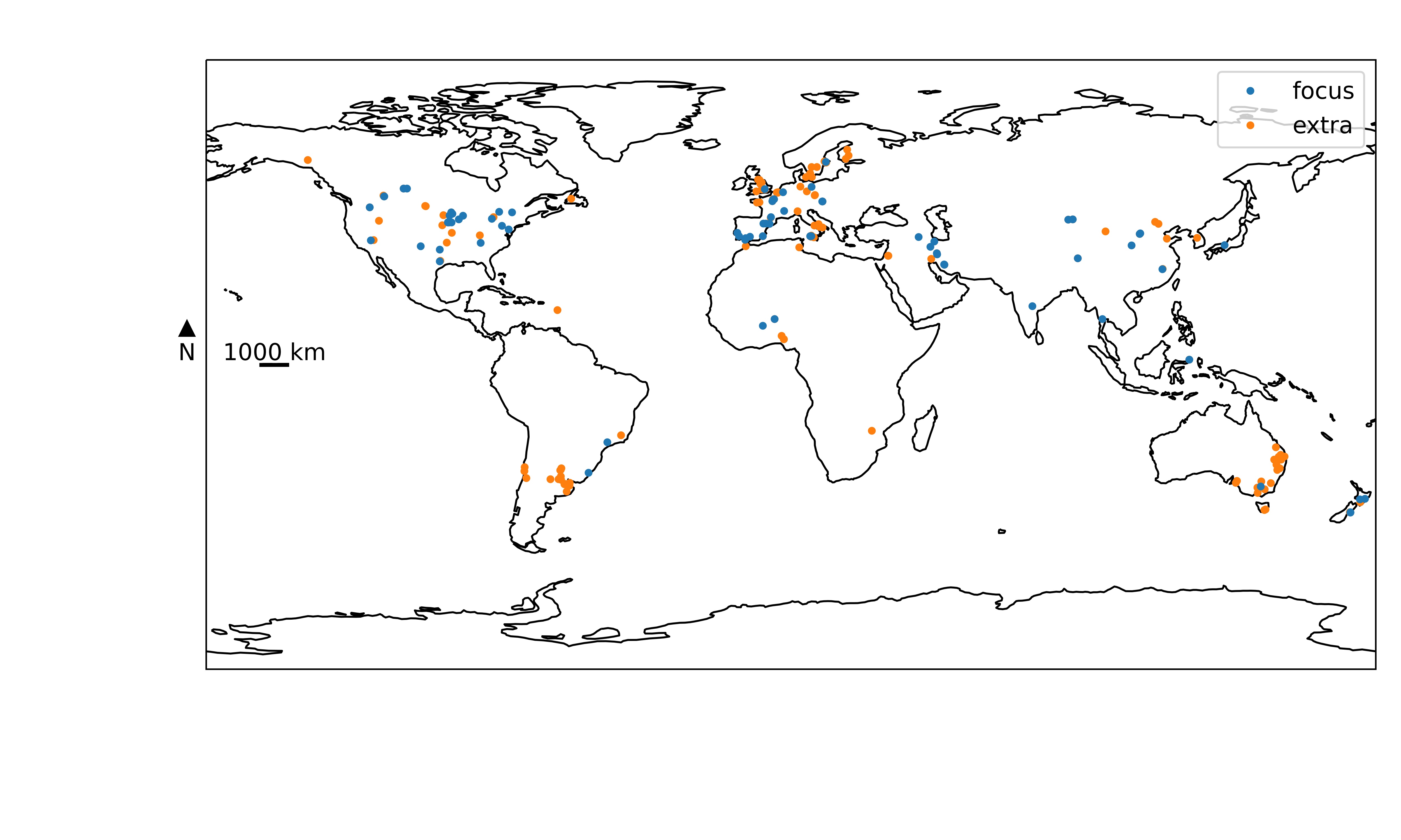
Map of the study locations collected in the OTIM-DB. See caption to Figure 3 for the definition of ‘focus’ and ‘extra’ locations.
Figure 5 depicts the number of Kh values available for 0 ≤ h ≤ 100 mm. These figures represent the hydraulic conductivities derived from the log-log linear model presented above, not the raw data measured and reported in the source publications. While a large number of entries span the full range of tensions of interest (0 to 100 mm), there are fewer entries that have data up to a tension of 60 mm. Often, but not always, such data series were obtained with the widely available Mini-Disk infiltrometer distributed by the Meter group (formerly by Decagon), which is limited to tensions h ≤ 70 mm.
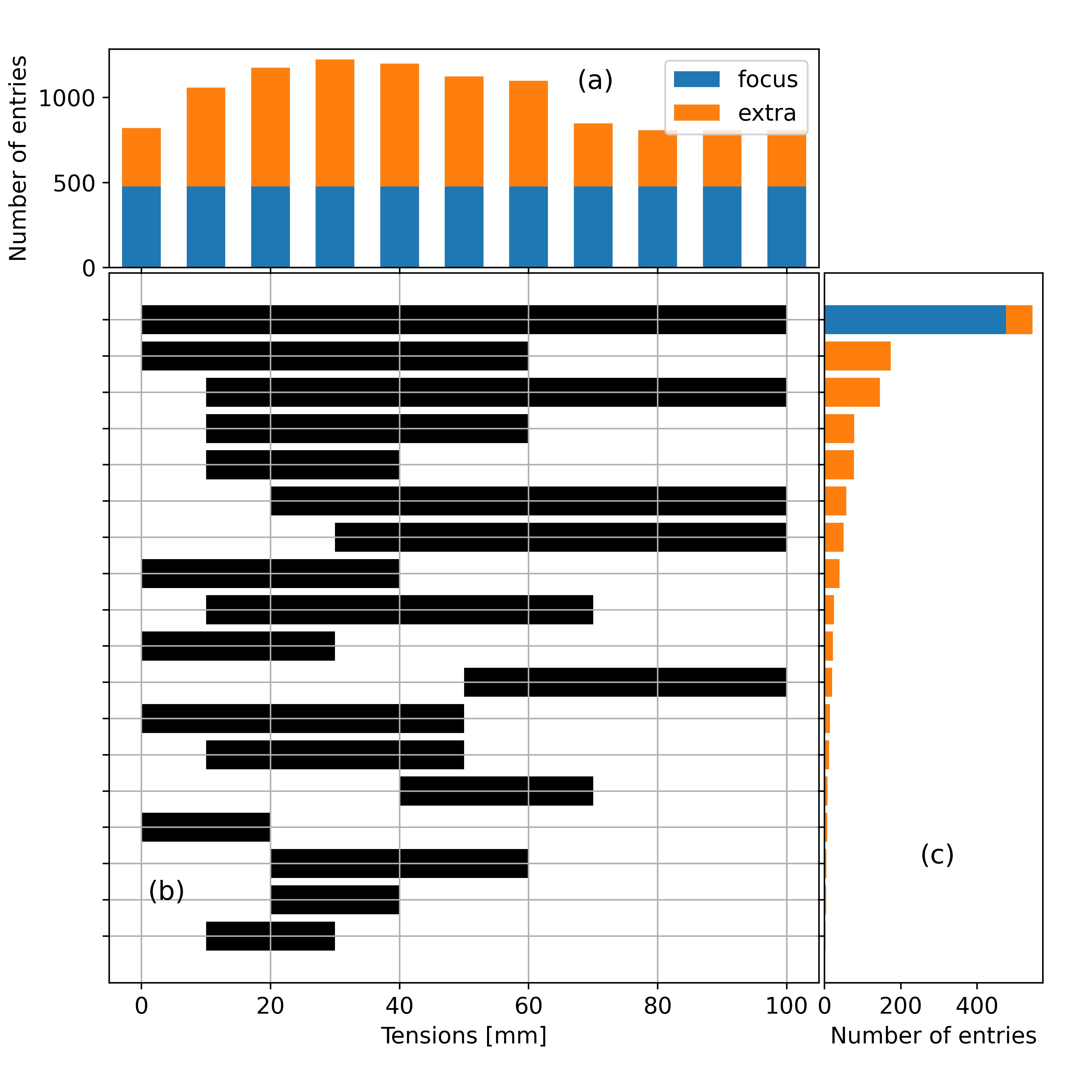
(a) number of available Kh values per supply tension, (b) range of available tensions and (c) their respective occurrence in the database.
An overview on the metadata included in OTIM-DB is given in Table 2. Data gaps are present, especially for bulk density and for information on the soil management at the study site except for tillage operations. Note that the annual mean temperature and precipitation are only two examples representing the climatic variables enumerated in section 2.3. There are very few missing values for the climate data, since it was estimated from the coordinates of the study sites. The same holds for the elevation data and information on the WRB soil type.
Number of entries and gaps for each feature along with units and range (if continuous) or choices (if categorical). The values are shown for the filtered entries (‘focus’) and in parenthesis for all the entries available in the database (‘focus’ and ‘extra’).
Type | Predictor | Unit | Range | Number of entries | Number of gaps |
|---|---|---|---|---|---|
Soil | Sand content | kg.kg-1 | 0.0 -> 0.9 (0.0 -> 1.0) | 369 (1070) | 40 (215) |
Soil | Silt content | kg.kg-1 | 0.0 -> 0.8 (0.0 -> 0.8) | 369 (1070) | 40 (215) |
Soil | Clay content | kg.kg-1 | 0.0 -> 0.7 (0.0 -> 0.8) | 372 (1107) | 37 (178) |
Soil | Bulk density | g.cm-3 | 0.5 -> 1.8 (0.1 -> 2.2) | 302 (771) | 107 (514) |
Soil | Soil organic carbon | kg.kg-1 | 0.0 -> 1.0 (0.0 -> 1.0) | 320 (938) | 89 (347) |
Climate | Annual mean temperature | °C | -3.8 -> 27.9 (-3.8 -> 29.1) | 409 (1214) | 0 (71) |
Climate | Annual mean precipitation | mm | 22.0 -> 3183.0 (22.0 -> 3183.0) | 409 (1214) | 0 (71) |
Climate | Average aridity index | 0.0 -> 1.9 (0.0 -> 2.8) | 409 (1214) | 0 (71) | |
Climate | Precipitation seasonality (CV) | 9.9 -> 111.2 (9.6 -> 138.5) | 409 (1214) | 0 (71) | |
Climate | Mean diurnal range | degC | 6.9 -> 18.2 (4.8 -> 18.5) | 409 (1214) | 0 (71) |
Management | Land use | choices | arable, bare, grassland, woodland/orchard | 396 (1249) | 13 (36) |
Management | Tillage | choices | conventional tillage, no tillage, reduced tillage | 384 (1190) | 25 (95) |
Management | Soil compaction | choices | compacted, not compacted | 62 (265) | 347 (1020) |
Management | Sampling time | choices | after tillage, consolidated soil | 324 (993) | 85 (292) |
Meta-analyses
Methods
Exploratory data analysis
Some source publications only provided a few data entries for Kh, sometimes only comparing two different treatments, while other source studies contain data for a larger number of treatments and/or sites. In some publications, data for all individual tension-disk measurements are available, even if replicates were measured. In others, only averages of the replicated measurements are reported, while still others yield average Kh values for individual replicated treatment blocks. This makes appropriate data weighting complicated, but also extremely important when analysing the meta-dataset. It also introduces uncertainty, because it is not always clear whether the replicated averages were calculated using the geometric or the arithmetic mean. Considering that hydraulic conductivities at or near saturation are known to be log-normally distributed, the former would be best. In the following, we assumed that geometric averaging was used when replicated values were reported in source publications. In the following, we calculated data weights as
where ωi is the weight for data entry i, nr,i is the number of replicates from which the values of i were averaged and Ni is the total number of measurements included in the publication from which data entry i was obtained. With the above described weights, we up-weight data entries according to the number of replicate measurements from which they were averaged, but down-weight the impact of studies that published larger amounts of data.
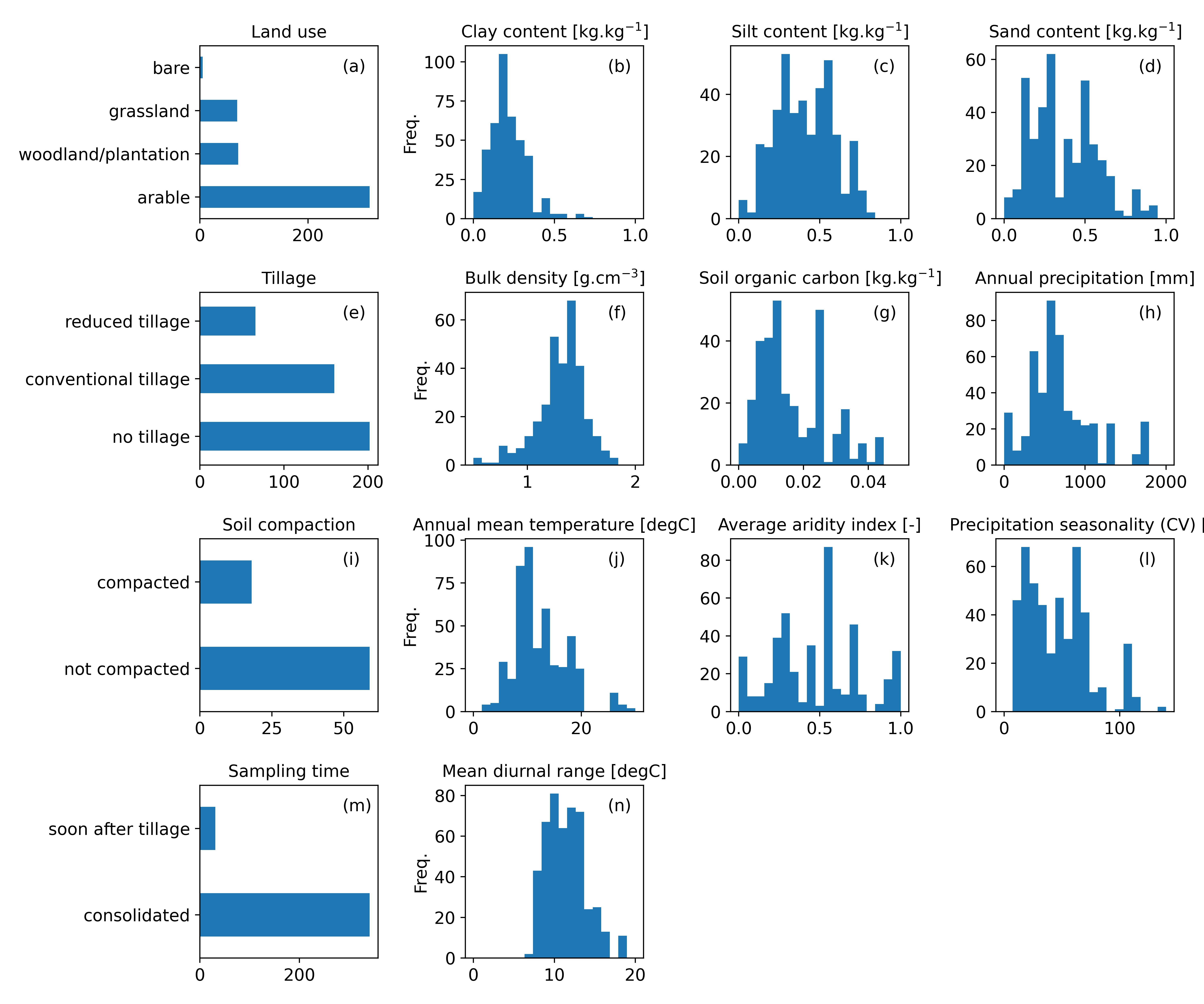
The metadata for the datasets used in the exploratory data analysis are summarised in Figure 6. The distributions of the climate variables illustrate that the data in OTIM-DB was mostly acquired in temperate climates, with a bias towards drier climates, as already expected from the distribution of the sampling sites shown in Figure 4. The soil texture, bulk density and organic carbon content data appear reasonably representative for soils in this climate zone. OTIM-DB contains predominantly data from arable fields.
Effect size computation
Data entries in OTIM-DB with specific land use or management were very unevenly distributed. For example, the large majority of data was measured on sites with land use ‘arable’ (see Figure 6a). Such uneven distributions may lead to bias when it is averaged over all entries of a specific feature like it was done in the exploratory data analysis. We therefore investigated the effects of land use and management as well as soil compaction and time of measurement on Kh with the aid of pairwise comparisons published within individual studies and calculated so-called effect sizes (ES) for each investigated feature class.
To reduce bias arising from the varying number of data entries published within individual studies, we grouped all entries according to the factors land use, tillage, compaction, and sampling time. Here we only considered binary pairs, that is arable or not arable in the case of land use and tilled or not tilled, compacted or not compacted as well as ‘measured soon after tillage’ or ‘measured on consolidated soil’ for the other three factors. In addition, we checked whether different entries within individual studies stemmed from the same or a very similar site. We did this by comparing the respective USDA texture classes and a climate variable, namely the aridity class. All data entries within an individual study that exhibited identical land use, soil management, compaction, sampling time, texture and aridity were averaged and the number of corresponding replicates was summed.
For each binarized factor (e.g. Tillage), a control value was chosen (e.g. zero tillage). All values different from the control represent the treatment (e.g. conventional tillage and reduced tillage). Within individual studies, pairs among the averaged entries were formed for each combination of a control and a treatment value. These pairs were used to compute the effect size. Following Basche & DeLonge (2019), we defined the effect sizes as the log10 of the ratio of Kh,t of the treatment divided by Kh,c of the control
where the subscript indicates the lth pair for which the effect size was computed and the indices ‘t’ and ‘c’ stand for treatment and control, respectively. The average effect size ES for each of the four investigated factors was calculated as the weighted mean of the individual ESl using the weight
where the subscript l indicates again the lth pair for which the effect size was computed and and denote the number of (summed) replicates for control and treatment, respectively. In addition, we calculated the weighted standard error
where is the mean effect size.
Table 3 summarises the evaluated factors, the number of pairs involved and the number of different studies from which the pairs were obtained.
Number of studies and paired comparison with their respective control and treatment values used for the meta-analysis of K10 values.
Factor | Control | Treatments | Studies | Paired comparisons |
|---|---|---|---|---|
Land use | not arable | arable | 10 | 24 |
Tillage | no tillage | conventional tillage, reduced tillage | 15 | 32 |
Compaction | not compacted | compacted | 6 | 8 |
SamplingTime | consolidated soil | soon after tillage | 6 | 12 |
To estimate the robustness of the effect size, we carried out a sensitivity analysis using the Jackknife technique, similarly to Basche & DeLonge (2019). This method aims to show the sensitivity of the averaged effect size to data from specific studies. For each factor, a given number of studies was randomly picked and removed from the dataset. The averaged effect size and its standard error was computed with the rest of the dataset. The process started by removing one study, after which up to nine more studies were removed. This random picking was repeated 50 times to rule out bias. The average of the means and standard errors for the 50 realisations was computed and plotted. Observed effect sizes were judged trustworthy, if they did not change after removal of studies to calculate them. We constrained the sensitivity analyses in our study to the effect sizes for Ks and K100.
Publication bias
We planned a publication bias following the procedures summarised in Rothstein (2005). The analytical sequence to be used was: i) the graphical method of contour-enhanced funnel plots, which help to relate asymmetry patterns to statistical significance; ii) the assessment of the small-size effects with the Egger’s regression test; iii) the trim and fill method to assess and to correct any asymmetry in the funnel plot; iv) the p-curve method, which focuses on p-values as the main driver of publication bias.
As suggested in the literature, in the application of this sequence we planned to use two threshold values for the implementation of the analytical pathway: the presence of at least ten studies with the required starting information and a heterogeneity value of less than 50% to apply of the trim and fill and the p-curve methods. In the analytical sequence, we instead excluded the application of the Failsafe N method because it ignores the magnitude of the effect, and no statistical criteria were available to aid interpretation.
The information required at the outset for the publication analysis is the value of the effect sizes together with their standard deviations for each of the studies selected in the meta-analysis. Unfortunately, most of the selected publications did not report dispersion statistics in numerical form or in any way derivable from the figures. For example, in the case of the conventional tillage vs. no tillage comparison, only 8 of the 24 studies reported standard deviations of effect sizes, while only two of them reported the standard deviations of the log-transformed values that would be needed to estimate the publication bias as outlined above. Failure to meet this basic requirement prevented us from proceeding in more advanced publication bias analysis.
However, we carried out a simpler approach for the K100 data, in which histograms of the response ratios were investigated. Any deviation from a normal distribution indicates publication bias.
Results and discussion
Differences between data entries with different tension ranges
If all data are considered (‘focus’ and ‘extra’), Figure 5 illustrates that approximately 40% of the data in OTIM-DB provided Kh for every h with 0 ≤ h ≤ 100 mm. For another 40%, Kh was only measured in the wet range, i.e. at tensions below 70 mm. The remaining Kh data was only acquired at the dry range. Here, we counted all data entries for which Ks were not measured and could not be estimated. Figure 7 illustrates how data from entries with complete, dry and wet ranges differed. The Kh for the wet range receded faster with increasing tension than series that also included measurement in the dry range. A large portion of these datasets were obtained with the Mini-Disk infiltrometer. However, a closer inspection of the impact of the disk diameters used to acquire the respective Kh did not confirm suspicions that the bias was related to the use of this special type of infiltrometer. While the observed differences between the Kh curves could have been introduced by co-correlations with soil texture or climate, other explanations appear more plausible. The vast majority (approximately 86%) of the experiments in OTIM-DB were conducted starting from a high tension and progressively measured at more saturated conditions. It follows that the first measurement of Kh series including large tensions was carried out under drier conditions than the series focusing only on the wetter range of the spectrum, respectively. The larger the supply tension, the longer it takes to acquire a measurement. It may therefore be that any initial water repellency of soils played a major role when the experiments were started under relatively wet conditions, while it was overcome during the first infiltration run under drier conditions. Another potential explanation would be that the steeper Kh recessions with tension for the data series in the wet range were caused when fitting the log-log linear model. If this was the case, it would follow that the log10 Kh to log10 h slope was steeper for smaller than for larger tensions, thus deviating from a linear relationship. Whatever the reason behind this observation, we found that including the data series that are constraint on the wet tension range leads to artefacts in Kh relationship with tension, which take on the form of a kink in between tensions of 60 and 70 mm. Note that similar kinks were when mixing data from data entries for which Kh had only been measured at the dry end of the considered tension range. Also already discussed, we focused solely on data entries for which we were able to reconstruct Kh for all h in between 0 and 100 mm supply tension in the following exploratory data analyses and meta-analyses. This greatly facilitated the data interpretation.
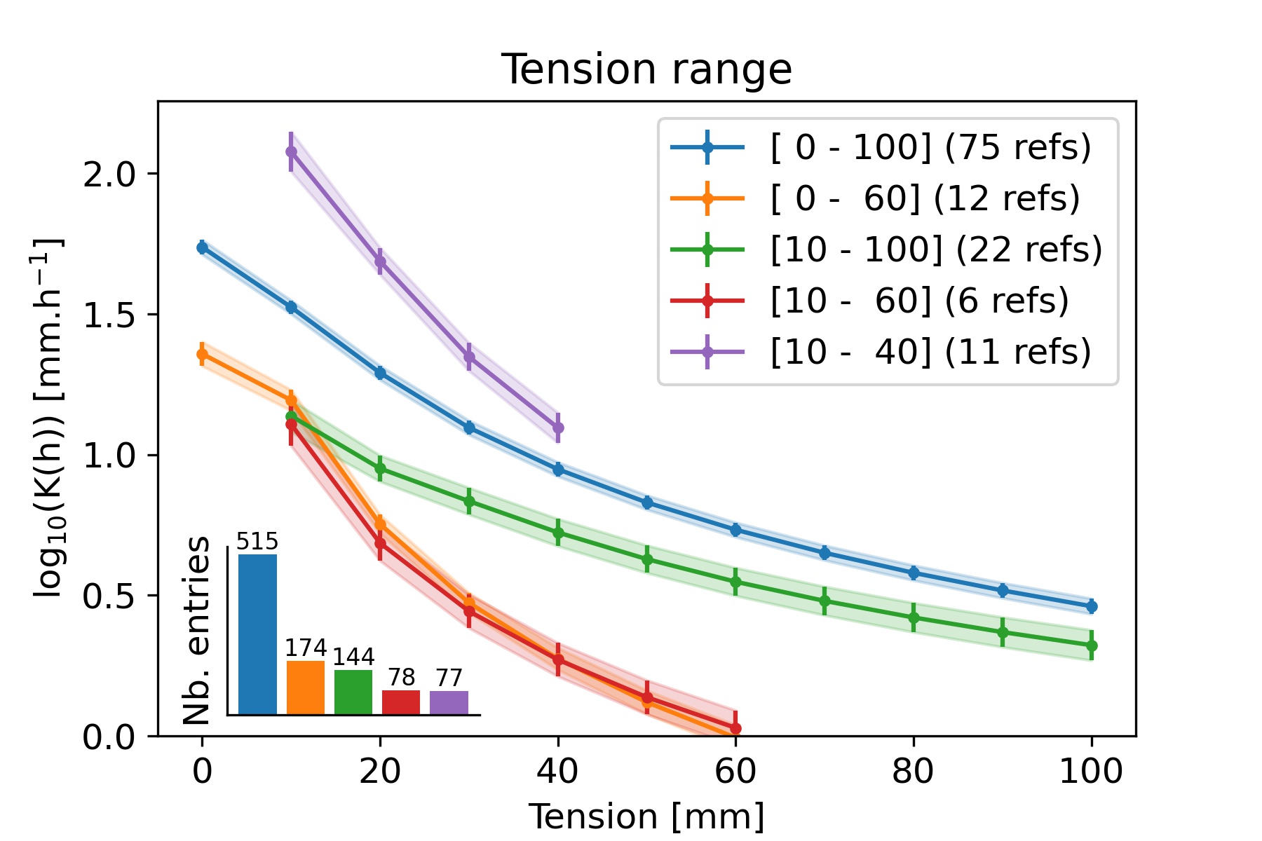
Evolution of weighted mean *Kh *with tension available in OTIM-DB, sorted by the tension range the data was spanning. The number of publications from which the data originated is shown between parentheses in the legend. The shaded areas and the error bars represent the weighted standard error of the mean.
Statistical relationships between Kh and methods used
Figure 8a confirms that the diameter of the tension disk did not have a systematic impact on the results. The majority of the data were collected starting under dry conditions (large tensions) and subsequently measured under increasingly wet conditions (smaller tensions). Figure 8b illustrates that beginning the experiment under wet conditions is associated with larger water contents and hydraulic conductivities at identical supply tensions. This is well known and referred to hysteresis, which is due to ink bottle effects, impacts of water repellency, air entrapment and swelling of clay particles Hillel, 2003. Figure 8c shows that the large majority of studies used the ‘steady-state piecewise’ method to solve the Wooding equation and convert the measured infiltration rates to hydraulic conductivities. This method leads to smaller Kh for larger tensions than the other methods. The ‘transient’ and ‘steady-state constant’ methods yielded larger Kh in the unsaturated range. For the latter method, it is known that it overestimates unsaturated Kh Jarvis , 2013. We tested whether excluding data from ‘transient’ and ‘steady-state constant’ methods changed the results of the meta-analyses, but found that they only changed to a minor degree. Data from all methods were therefore included in the following. Note that the ‘transient’ method was mostly applied in conjunction with Mini-Disk Infiltrometers, albeit the respective data is not included in Figure 8 since it does not span the entire suction range.
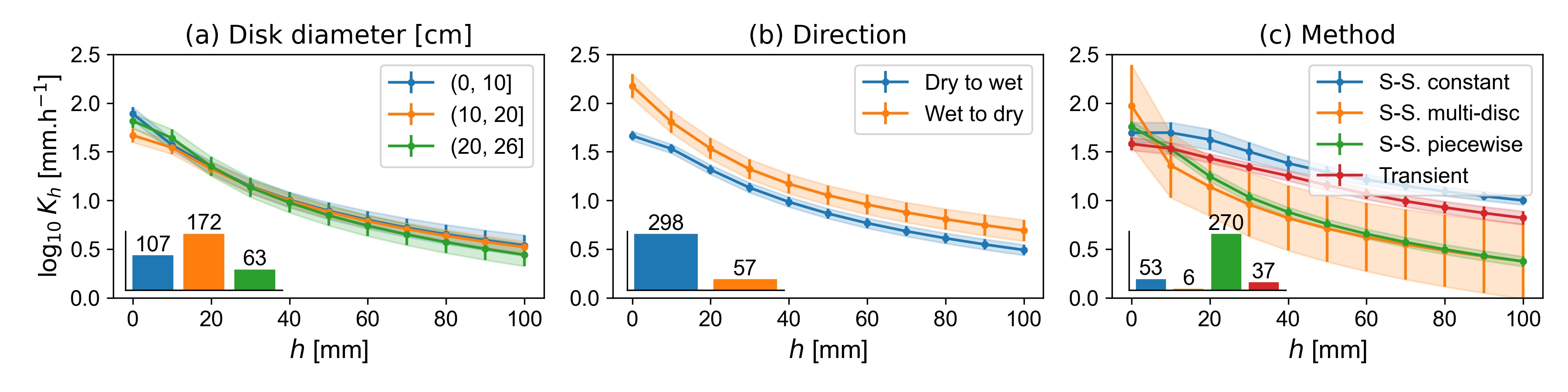
Evolution of weighted mean *Kh *as a function of applied tension for (a) disk diameter, (b) direction and (c) method of fitting. ‘S.-S.’ stands for ‘steady-state’. More specifically, the method ‘S.-S. constant’ is outlined in Logsdon and Jaynes (1993), ‘S.-S. multi-disc’ in Smettem and Clothier (1989), and ‘S.-S. piece-wise’ in Reynolds and Elrick (1991) or Ankeny (1991) and ‘Transient’ in Zhang (1997) or Vandervaere et al. (2000). The shaded areas and the error bars represent the weighted standard error of the mean.
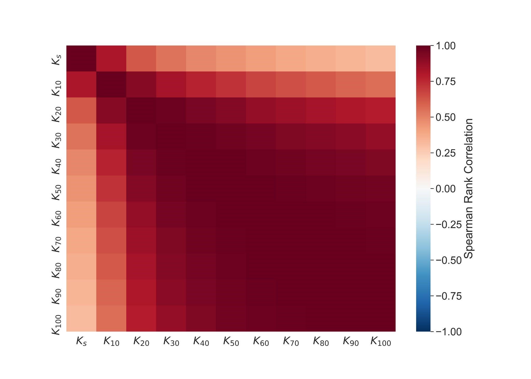
Correlations between Kh at different saturations
Figure 9 illustrates that Ks was clearly different from Kh in the near-saturated range. Already K10 was better correlated with K20 than with Ks. This indicates that Ks results from fundamentally different flow paths than Kh at 20 mm supply tension or drier. The flow paths at saturation reflect the largest connected macropores. Also air entrapment may play a role here. It may alter the relationship between pore-network morphology and water-flow paths and therefore further decouple Ks from proxies describing the pore-network. Figure 9 also shows that Kh was strongly correlated in the range between 40 and 100 mm tensions. This indicates that flow paths did not dramatically change with tension at the dry end of the investigated tension range.
Statistical relationships between Kh and soil properties
Soils with coarse texture exhibited larger Kh in the unsaturated range, which is caused by the large and abundant primary pores in between individual sand grains (Figure 10a). At saturation, the hydraulic conductivity of all three texture classes was approximately identical. This is explained by the presence of large structural pores in the medium and fine-textured soils. Medium-textured soils had the lowest Kh in the investigated range of tensions, which may be due to a denser soil matrix in loamy soils and a lower structural stability of silty soils. Larger bulk densities decreased Kh across the whole range of investigated tensions, which reflects the reduced porosity with increasing bulk density (Figure 10b). The hydraulic conductivity in the saturated and near-saturated range is especially affected by soil compaction, which predominantly reduces the abundance and connectivity of macropores Pagliai , 2004Whalley , 1995. Large bulk densities are also known to reduce burrowing activities of the soil macrofauna Capowiez , 2021 as well as root growth Lipiec & Hatano, 2003, also leading to less abundant and less connected large macropores. The soil organic carbon content was connected with smaller Kh at the dry end of the investigated tension range if soils with organic carbon contents of more than 0.03 kg.kg-1 were excluded (Figure 10c). This decrease may be explained by water repellency, which is generally positively correlated with organic carbon content. A similar observation was already reported in Jarvis (2013). Note that correlations of SOC with soil texture were not observed in the investigated dataset (Figure 11).For soils with organic carbon contents larger than 0.03 kg.kg-1, Kh increased once again. This may indicate that, above this threshold, better developed macropore networks associated with large SOC contents (e.g. Larsbo (2016)) outweighed any effects of water repellency.
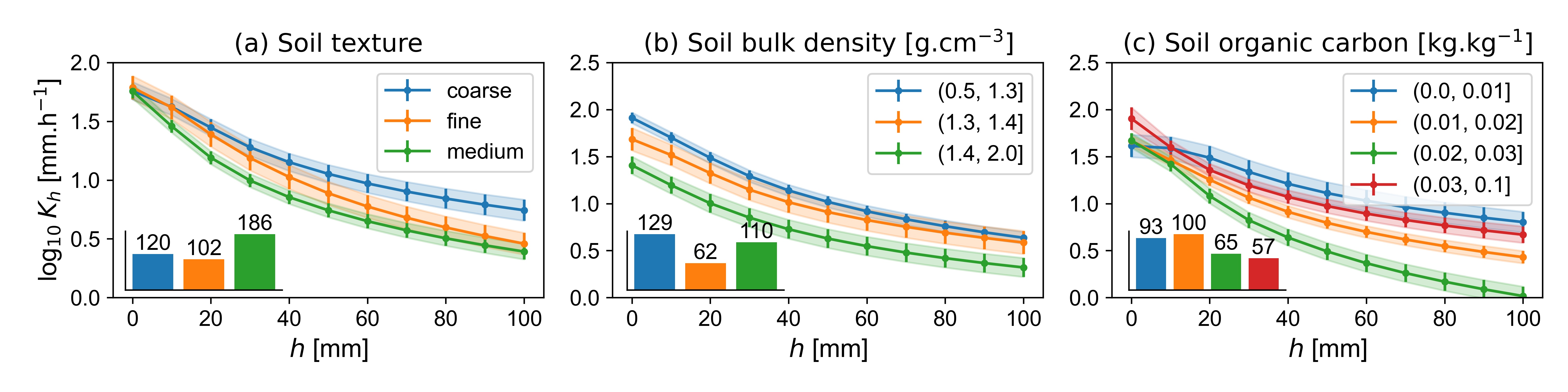
Evolution of weighted mean Kh as a function of applied tension for (a) soil texture, (b) soil bulk density and (c) soil organic carbon. The shaded areas and the error bars represent the weighted standard error of the mean. The soil textures were classified using USDA texture classes as follows: fine (clay, clay loam, silty clay, silty clay loam), medium (silt loam, loam), coarse (loamy sand, sand, sandy clay, sandy clay loam, sandy loam).
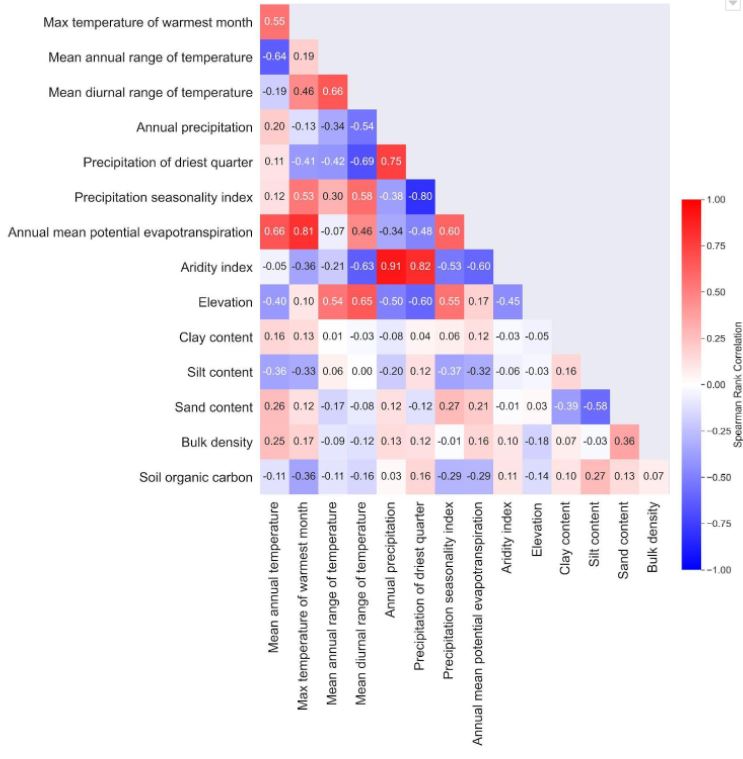
Weighted Spearman rank correlation coefficients between climate variables, elevation above sea level and soil properties.
Statistical relationships between Kh and climate variables
One of the important observations made in recent years was that saturated and near-saturated hydraulic conductivities are strongly correlated with climate variables Jarvis , 2013Jorda , 2015Hirmas , 2018. Figure 11 gives an overview over weighted Spearman rank correlations between Kh and nine of the 20 climate variables included in OTIM-DB that exhibited the strongest correlations with Kh. The elevation of the sampling site above sea level, its latitude and the values for soil texture, bulk density and soil organic carbon content are also shown for comparison. It is striking that the soil properties were clearly less well correlated with Kh than some of the climate variables. The largest absolute values of the weighted rank correlations were observed for the mean diurnal range of temperature and the aridity index. Both reach a maximum at the dry end of the considered tension range, i.e. for K10, with correlation coefficients of 0.54 and -0.47, respectively. The strength of these correlations was reduced with smaller tensions to values close to zero at Ks (Figure 12). The loss of correlation occurred rather abruptly at supply tensions between 10 and 20 mm, again pointing at a threshold above which different kinds of pores and/or air entrapment may become important for water transport.
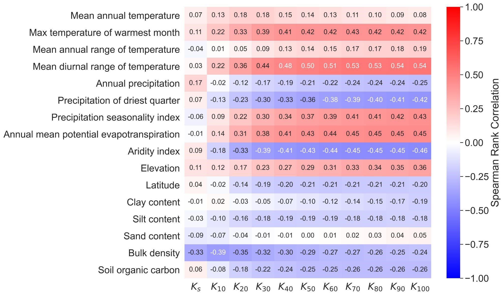
Weighted Spearman rank correlation coefficients between Kh at different tensions and selected climatic features, the elevation above sea level as well as soil properties. The soil textures were classified using USDA texture classes as follows: fine (clay, clay loam, silty clay, silty clay loam), medium (silt loam, loam), coarse (loamy sand, sand, sandy clay, sandy clay loam, sandy loam).
It should be noted that both variables, the annual mean diurnal temperature range and the aridity index, were strongly correlated with each other, with a weighted correlation coefficient of 0.67 (Figure 11). Strong correlations to at least one of these two variables with absolute values >0.6 were also found for most of the investigated climate variables. It is difficult to separate the climate effects due to these strong inter-correlations. But it stands out that not only the mean annual diurnal temperature ranges are much better correlated with K100 than the mean annual temperature itself. Also the mean annual precipitation in the driest quarter of the year and the precipitation seasonality index exhibited stronger correlations than the mean annual precipitation. It appears that temperature and precipitation fluctuations are more strongly coupled to near-saturated hydraulic conductivities than the absolute temperatures or precipitation amounts. In the following we attempt an explanation.
Larger diurnal temperature ranges may lead to larger near-saturated hydraulic conductivities because it might stimulate migration of soil macrofauna between topsoil and subsoil to prevent excessive heating or cooling. Burrow systems may therefore extend more in the vertical than the horizontal directions and reach further into the subsoil. Moreover, frequent large temperature shifts may be associated with larger changes in moisture conditions due to dew formation and subsequent evaporation. It also is connected with more frequent freezing thawing cycles. The correlation may also partly be driven by the moderating effect of large soil moisture contents on the diurnal temperature range. Soils with low Kh are expected to dry slower than soils with large Kh. Wet soils heat and cool more slowly than dry soils, because water has a large heat capacity and the phase changes occurring during evaporation or condensation add to decreasing the rate at which the soil heats up. Hence, small Kh buffer diurnal temperature shifts. It is not clear to what extent the observed correlation was driven by high diurnal temperature ranges causing high Kh or, the other way around, low Kh led to low diurnal temperature ranges.
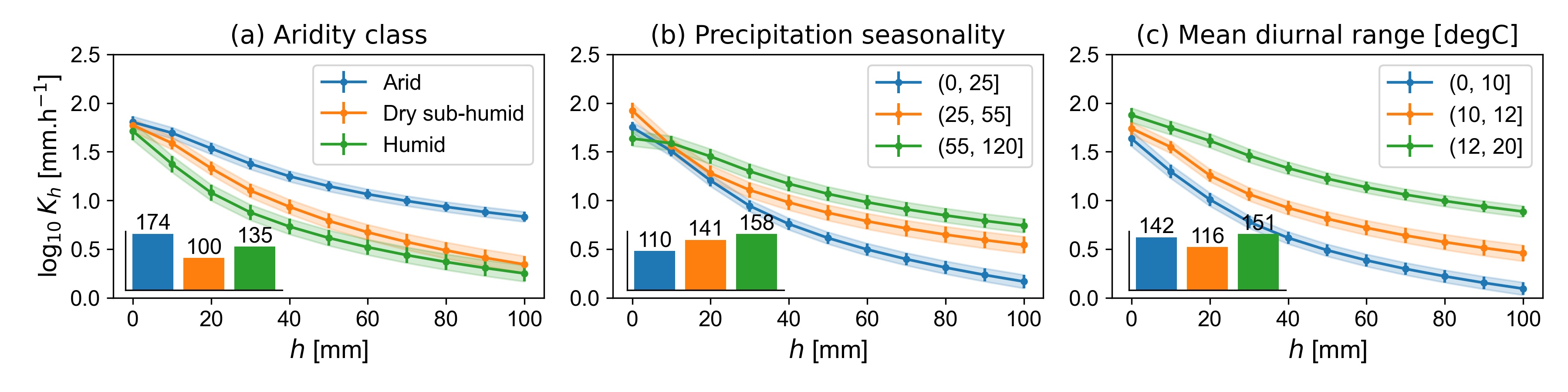
Weighted mean *Kh *as a function of applied tension for (a) aridity classes, (b) precipitation seasonality and (c) mean diurnal temperature range. The shaded areas and the error bars represent the weighted standard error of the mean.
The negative correlation between aridity index and Kh, i.e. the drier the climate, the larger Kh, is more intuitive. Dryness forces plants to grow deeper roots. It also forces the soil macrofauna to burrow deeper into the soil to prevent drying out. This creates vertical connected macropore systems which increase Kh. Large precipitation seasonality may contribute to larger Kh, because they indicate the presence of dry seasons, under which the topsoil dries out thoroughly, which may stabilise existing macrostructures in soil.
Another site factor that is positively correlated with Kh is the elevation above sea level (Figure 13). In the case of infiltrometer measurements, the decreased atmospheric pressure with height on the supply tension can be neglected. The supply tension is always equivalent to the weight of the water column adjusted for the measurement. The weight of the water column will be smaller due to the general decrease of earth’s gravitational constant with height due to a larger centrifugal force. However, the weight of the water column would only be reduced by approximately one or two percent. Also, indirect influences of larger heights on the infiltration rate cannot explain the observed correlation. A lower temperature would make the water column heavier, however, the effect would be less than 1% in the relevant temperature range. In contrast, a lower temperature would increase the water’s viscosity to a much larger degree, e.g. by up to approximately 30% between temperatures of 10 and 20 oC. The temperature effect should thus lead to a negative correlation between elevation and Kh, which is the opposite of what was observed. Physically explainable bias in the Kh measurements can thus be ruled out. The elevation may instead be a proxy for well-drained soils, as stagnant soil water and high groundwater tables are less likely with height above sea level. This may favour soil life and better developed root systems. Notably, the elevation above sea level also was found to be an important predictor for Ks in Gupta (2021), which suggests that there are indeed pedogenetic reasons behind the observed correlation.
Bulk density was the only soil property that exhibited (negative) correlation strength of > 0.3 to any Kh (Figure 13). The underlying reasons have been discussed above. Notably, the strongest correlations were found at and very close to saturation due the direct link between bulk density and macroporosity. The more compaction, the less macroporosity remains and the higher the bulk density. In addition, this then again negatively impacts the options for root growth and bioturbation.
Effects of land use, tillage, compaction and sampling time
Figure 14 shows the average log10 response ratio of Kh for 0 ≤ h ≤ 100 mm for different land uses and soil management options. Arable land exhibited clearly smaller Ks than grasslands and forests, which is in line with observations made by Basche & DeLonge (2019). This difference became smaller with higher tensions (Figure 14a). The large difference in Kh close to saturation was likely related to traffic compaction as well as tillage operations that were applied to the majority of the investigated arable soils, which lead to the destruction of connected biopores and hence a reduced Ks. On the other hand, tillage breaks up intact soil into individual soil aggregates, which creates, at least initially, a well-connected network of inter-aggregate pores that increase Kh in the near-saturated range Sandin , 2017Schlüter , 2020. This effect of tillage can explain why near-saturated Kh under conventional and reduced tillage was larger than under no-till (Figure 14b). However, in this case, even Ks was larger in the tilled fields. It is likely that Ks was reduced in the no-till treatments due to more trafficking on the fields as compared to non-arable treatments. The impact of soil compaction on Kh was clearly negative in the entire investigated range of tensions (Figure 14c), which is explained by the reduction of porosity, and especially the macroporosity during compaction (see also Figure 10b). In contrast, if the Kh measurements were carried out shortly after tillage operations, Kh was increased for all investigated tensions, especially very close to saturation (Figure 14d). This confirms that tillage initially increases Ks, but that subsequent soil consolidation preferentially disconnects the largest macropores. As a consequence, Kh at and very close to saturation is reduced more strongly than Kh for higher tensions.
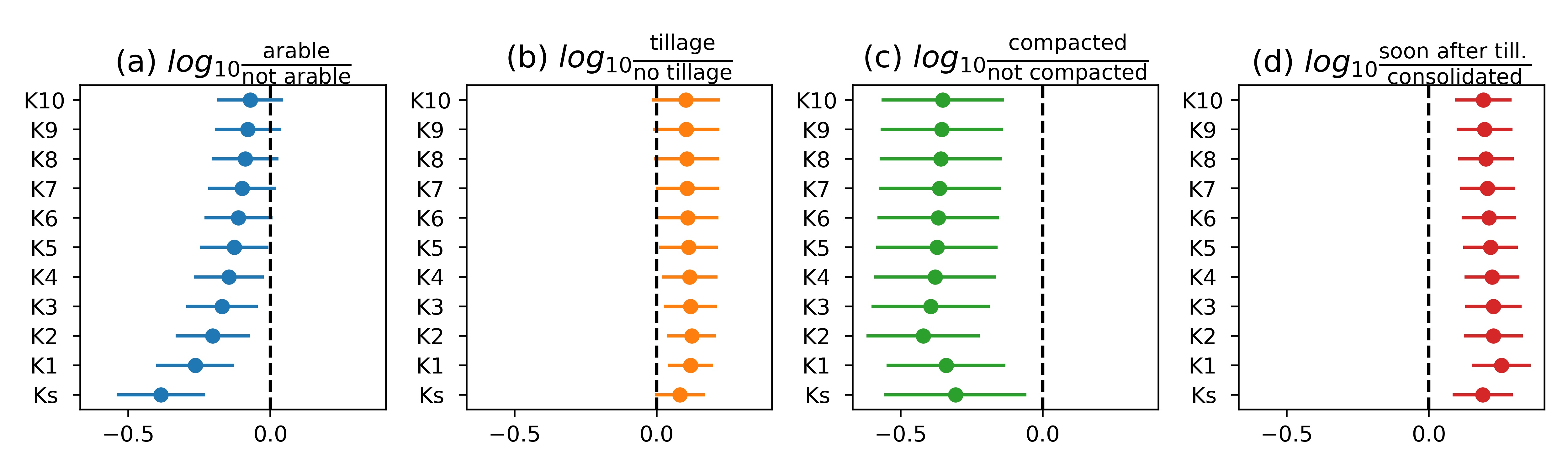
Weighted mean log10 response ratio (effect size) of Kh for from K100 to Ks for different management practises where the controls were ‘not arable’, ‘no tillage’, ‘no compaction’ and ‘consolidated soil’ respectively. Positive effect size means that the value of the treatment is greater than the control. Dashed line shows the “no effect” (no difference between treatment and control). Error bars represent the weighted standard error of the mean.
Figure 15 shows the results of the sensitivity analyses for the effect sizes depicted in Figure 14. The effect of land use for K100 turned out to be the most sensitive to removals of studies (Figure 15a). The direction of the effect even changed after removal of only two studies, indicating that higher K100 for arable compared to non-arable fields were not just occasional observations but occurred more frequently. More studies would be needed to properly characterise the effect of land use on K100. The sensitivity analyses for all other factors for both, K100 and Ks all yielded that removal of studies did not change or destabilise the results. The large majority of the respective studies in OTIM-DB had observed similar effects, thus validating them.
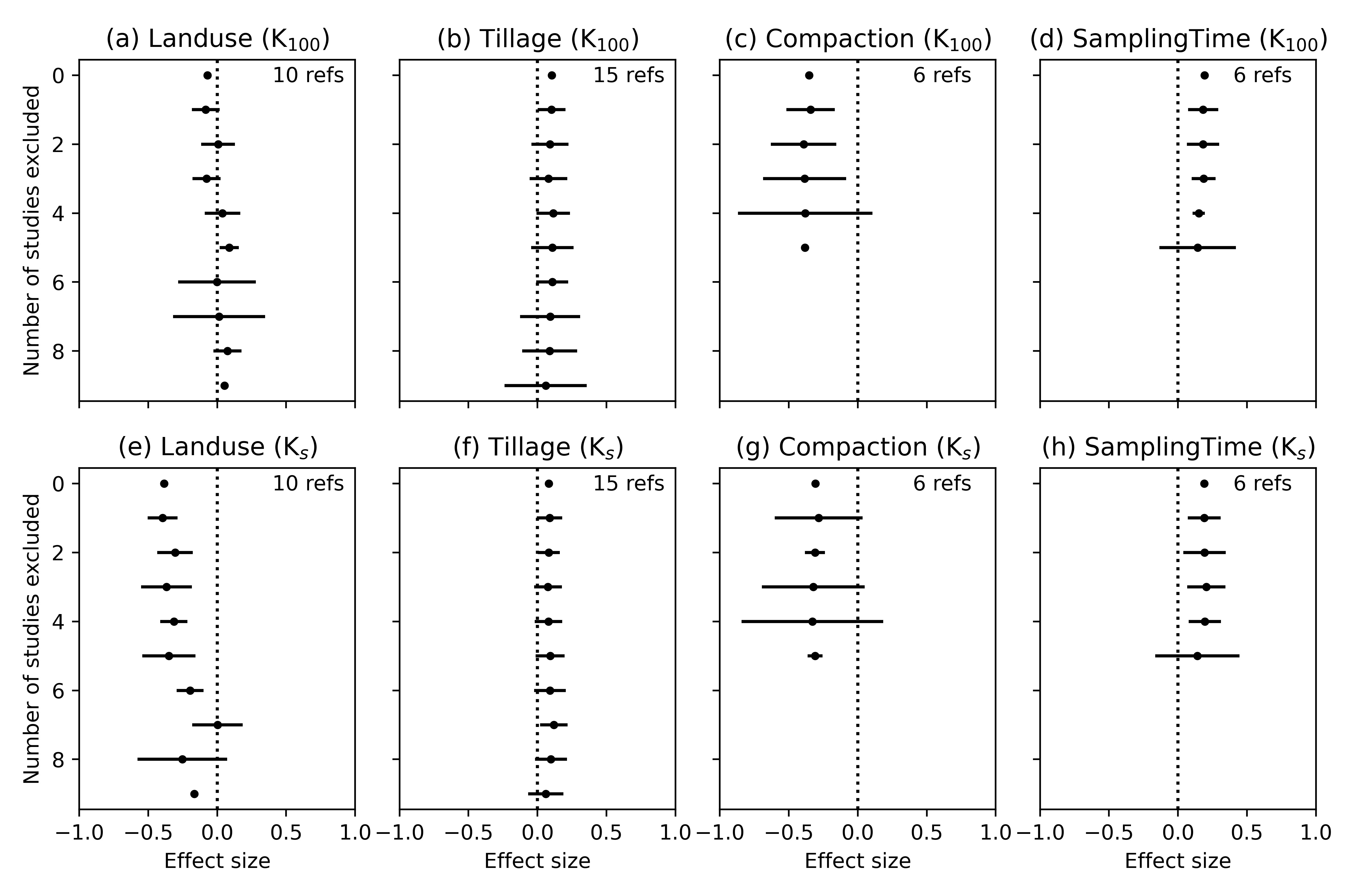
Sensitivity analysis of the weighted effect size of K at 100 mm tension and Ks for the management practice investigated using the Jackknife technique. The error bars represent the standard error.
Publication bias
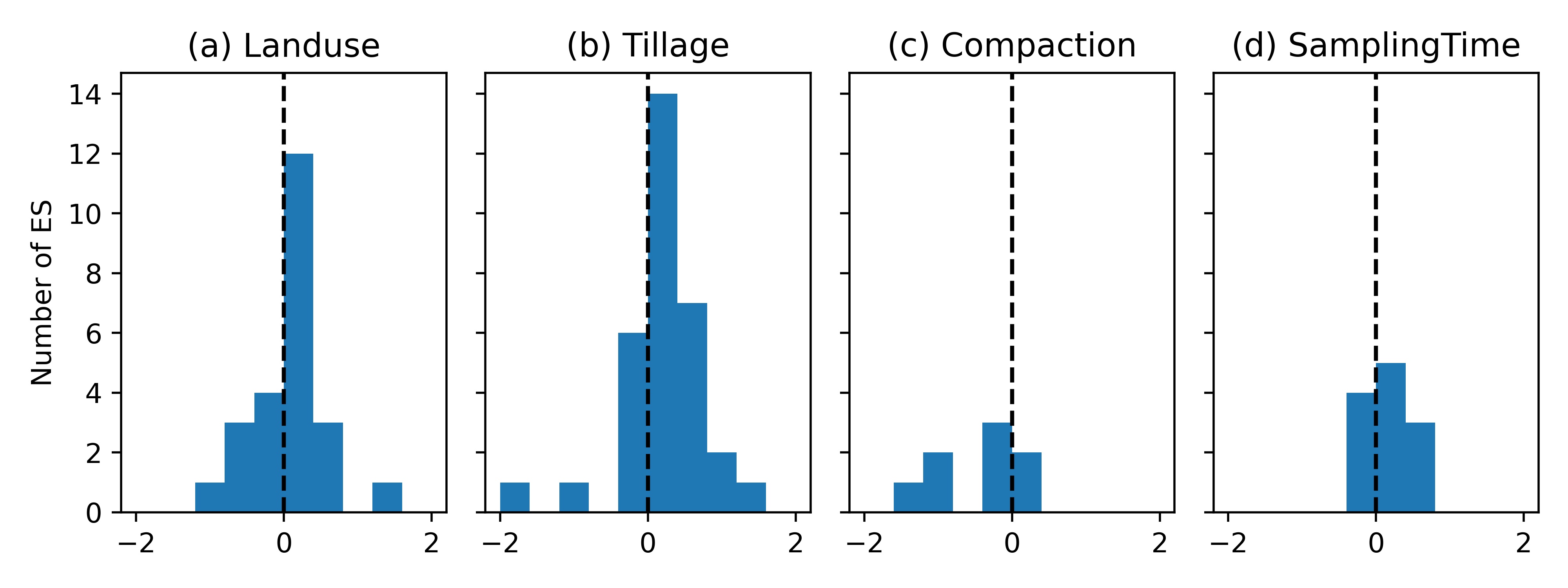
The histograms of the effect sizes for K100 are shown in Figure 16. For the tillage factor we observed a slight bias towards positive effect sizes, which may indicate publication bias, with more likely publications in case that conventional or reduced tillage yielded larger Kh than no-till. The small number of studies available in OTIM-DB to compute the effect sizes for compaction and sampling time makes it hard to obtain a smooth shape for the distribution and limits our ability to estimate bias for compaction and sampling time.
Conclusions of meta-analyses part
We observed the strongest correlations between climate variables and Kh, namely diurnal temperature range, aridity and precipitation seasonality. In the dryer range of investigated supply tensions, these correlations were clearly larger than correlation between Kh and soil properties like texture and organic carbon content. Our results suggest that climate change will influence soil hydraulic properties at and near saturation, complicating estimations for future risks of surface runoff with soil erosion and water-logging. On the one hand, this confirms the findings of Jarvis (2013), Jorda (2015) and Hirmas et al. (2018) that climate variables influence saturated and near-saturated soil hydraulic conductivity. On the other hand, the large positive correlation between K100 and the mean annual temperature reported in Jarvis (2013) on a part of the here investigated dataset was not found back. The importance of the above mentioned climate variables for Kh should be confirmed by additional measurement. Hypotheses of how these climate aspects influence Kh mechanically were presented in the results and discussion parts but need to be further investigated, as should be the large correlation of elevation above sea level to Kh.
At and very close to soil saturation, the correlation between Kh and the climate variables vanished. Instead, the soil bulk density showed the largest correlations. For this saturation range, land use and land management seemed to be more important, as tillage and soil compaction due to trafficking are known to lead to larger bulk densities. In this context we found that it is very important to take the time period after the last tillage into account, after which the tension-disk measurement was conducted, as larger Kh were measured shortly after tillage. Last but not least, our meta-analyses demonstrated that there is a need for better documentation and availability of measurement and associated meta-data. In our case, the lack of reporting standard deviations of the Kh measurements in log-space prevented a thorough analysis of potential publication bias. Missing information of land use and soil management and cropping practises and their history made it challenging to quantify their impacts on Kh. We therefore want to stress the need for better experimental documentations and open access to research data, as it has already demanded before McBratney , 2011Basche & DeLonge, 2019.
Machine learning
Material and methods
Machine learning approach: Light Gradient Boosting regression model
We used a tree-based model, namely the Light Gradient Boosting (LGB) regression model Ke , 2017, because this group of machine learning approaches allows for an easier interpretation of effects and importance of individual predictors. Tree-based machine learning models combine the predictions of decision trees using different styles of ensemble techniques. The term ‘boosting’ denotes a type of model that improves its predictions by giving samples with a large prediction error more weight in the fitting process with each training iteration. Usually, boosting methods outperform other tree methods. LGB is known to perform overall well for different machine learning tasks. The LGB model also performed best in preliminary trial runs on the OTIM-DB data. We used the lightgbm Python package (v3.2.1) to apply the LGB model to our data.
Data pre-selection and data weighting
As discussed, tree-based models are able to handle missing data. Nevertheless, too much missing information decreases the predictive performance of these models. For this reason, only predictors that contained at least 50% of the maximally possible number of data entries were considered for the modelling procedure.
We used the same weighting scheme as in the meta-analyses (see (1)) to avoid bias due to different amounts of entries over source publication and different number of replicates from which individual data entries were averaged.
Feature engineering
While tree-based methods are able to use categorical data without any transformation, we decided to encode all categorical values into numerical ones as then more information is provided for the model. For instance, tillage type was classified into three classes in OTIM-DB: conventional tillage, reduced tillage, and no-tillage. Assigning them values of 2, 1 and 0, respectively, allows classification on tillage intensity and not just on different tillage types. The conversion of the majority of categorical variables into numeric ones was carried out using Catboost encoding Prokhorenkova (2018), which is a type of target encoding. Target encoding assigns the average value of the target variable for specific entries of a categorical variable. For example, it replaces the categorical value ‘conventional tillage’ with the average Ks of all measurements on conventionally tilled sites in the database. A drawback of simple target encoding is that only three different values would become possible in the example of the tillage predictor as available in OTIM-DB. This does not favour selection of this variable in the LGB model. Catboost encoding uses averages of randomised subsets of all respective target values instead. As a result, a categorical variable with only two or three possible values is encoded into a continuous numeric variable with as many possible different values as there are unique data entries in the database.
We encoded the predictors ‘crop rotation’ and ‘season’ a different way. Crop rotations stored in OTIM-DB are very diverse. Almost each source publication reported a unique crop-rotation scheme. The individual crop-rotation schemes would therefore act as an identifier for a respective source publication. Therefore, it must not be encoded in with a simple Catboost approach. Another problem arises because for such a simple encoding, similar rotations e.g., maize-maize-wheat and maize-wheat would be classified as being completely different. Instead, we used a semi-one-hot encoding approach. In the original one-hot encoding, a new binary predictor is introduced for each unique entry of a categorical variable, which is one if the unique entry is true or zero if it is false. For semi-one-hot encoding, we classified the crops according to plant classes, e.g. cereals, fruit trees or grasses. Each of these subclasses held entries associated with this class like wheat, barley or oats for cereals. A new binary predictor for each subclass was created. It was filled with a one if one of the entries was contained in the underlying crop rotations and a zero otherwise. This procedure did not increase dimensionality drastically and introduced similarity within similar rotations. Afterwards, we encoded these new crop-class predictors using Catboost encoding to make them more suitable for the LGB model algorithm.
The cyclic predictor ‘season’ was encoded into two predictor
where S abbreviates the ‘season’ predictor, x (-) is the season with values of 0, 1, 2 and 3 for spring, summer, autumn and winter, respectively and xtot (-) is the number of seasons in a year, i.e. 4. This cyclic encoding conveys the information to the machine learning algorithm that spring is following winter.
Data imputation
Albeit that LGB can handle missing values, we filled data gaps using a random forest trained on the available data (Python package MissForest, Sekhoven & Bühlmann, 2011). This allowed us to use an advanced feature selection approach in the LGB hyper-parameter optimization (see below).
LGB training and validation
We used two different cross-validation schemes to train and validate the LGB model.
i) Naïve cross-validation
Naïve cross-validation denotes simple 10-fold cross-validation Hastie (2009). All available data entries were randomly assigned to ten different groups. We referred to the groups as folds in the following. We trained the LGB model on the data from nine of the folds and subsequently validated the trained model using the data of the remaining tenth group. Then, another fold was selected for validation and another LGB model was trained on the data from the respective remaining nine folds. This was done ten times in total, so that ten different LGB models were trained and a prediction was available for each data entry. The validation results of the naïve cross-validation reflect the predictive performance of the LGB model under the assumption that the dataset used to train it was a representative sample of the total statistical population. Considering the biassed and sparse distribution of sampling sites around the globe as well as the plethora of different possible influencing factors and the amount of gaps in the data collected in OTIM-DB, this assumption was most likely not met in our study. Therefore, it was expected that naïve cross-validation would result in over-optimistic validation results.
ii) Source-wise cross-validation
The source-wise cross-validation was already used in Jorda (2015). It is also a 10-fold cross-validation. However, this time, data entries of individual source publications were all contained in only one of the ten folds, respectively. The fold used for the model validation hence only included data-entries from studies that were unknown to the trained LGB model. Source-wise cross-validation hence simulates prediction of data from a new source. Its results are therefore realistic for applications of a final LGB model as a pedotransfer function. The source-wise cross-validation also resulted in ten LGB models and model predictions for each data entry.
Quantifying predictor importance
We used the SHAP (SHapley Additive exPlanations) importance to evaluate the importance of individual predictors on the model prediction Lundberg & Lee (2017). The SHAP importance is calculated by checking the difference of the model performance with and without a certain feature taken into account. Features that show a large predictive improvement when selected achieve a higher importance. SHAP values of a predictor quantify how much this predictor contributes to a prediction given a base value. The base value refers to the predicted target variable of the model without the predictor. For example, a predictor with a SHAP value of 0.2 mm.h-1 changes a prediction of the hydraulic conductivity from 1 mm.h-1 (base value) to 1.2 mm.h-1 (model prediction with the predictor). SHAP values increase the interpretability of predictor importance, since they provide a measure that quantifies the direction and the magnitude of the influence of the predictor on the target variable, expressed in the same units.
In the following, we investigated SHAP values based on the validation data of the source-wise cross-validation scheme. The SHAP value reflects the predictor importance to re-estimate the hydraulic conductivities presently stored in OTIM-DB. It must not be forgotten that the here discussed SHAP importance for predicting Kh has to be seen relative to the data in OTIM-DB from which it was derived. Only if the OTIM-DB data can be viewed as representative for Kh measurements in general, the SHAP importance is also generally valid. Otherwise, it will partly reflect biases in the OTIM-DB data.
When interpreting predictor importance of a machine learning approach, it also must be kept in mind that it depends not only on the data that was used to train the model, but also on the hyper-parameterization and the selected predictors (see next section). Quantifying these dependencies turned out to be too time consuming to be carried out within the framework of our study.
LGB model optimization including feature selection
Model optimization is a part of model training and is included in any machine learning workflow. It aims to enhance the results of a model and reduce computation time when making predictions. In our study, we carried out hyper-parameter optimization and feature selection. Hyper-parameters are parameters that govern the model building process. They need to be adjusted to minimise both, under and over-fitting. Common hyper-parameters of tree-based models are the number of branches used per individual decision tree or the total number of trees used. For example, trees with many branches are prone to overfitting. Trees with insufficient branches may not be able to represent the complexity of the fitted data, which would lead to under-fitting.
Feature selection describes an approach in which a subset of useful predictors is chosen from all available predictors to exclusively train the model. Usually feature selection increases the model performance slightly or at least does not worsen the prediction results, while it strongly reduces the required computational power. We applied the Boruta method described in Kursa & Rudnicki (2010), using the Python package BorutaSHAP. The method works by creating a so-called shadow predictor for each original predictor, which contains a random permutation of the values of the original predictor. The expected correlation of each shadow predictor with the target variable is therefore zero. We then trained an LGB model with both, original and shadow predictors. Each predictor whose SHAP importance for the model was smaller than the SHAP importance of the most important shadow predictor was deselected. Since this procedure depends heavily on the realisation of the random permutation of the original predictor values, the Boruta approach was performed 20 times using different random seeds. Only predictors were selected that were more important than the best shadow feature.
Because hyper-parameters influence feature selection and vice versa, we used an iterative approach to implement both. Here, a first optimization of the most basic hyper-parameters was performed using all predictors. We used the Python package Optuna Akiba , 2019 to carry out the hyper-parameter optimization. Optuna uses a tree-structured Parzen estimator for predefined discretized values within predefined boundaries for individual hyper-parameters. The model hyper-parameters were optimised to reduce the root mean squared error (RMSE) of either the naïve or the source-wise cross-validation scheme. From trial and errors, some hyper-parameters were found to not have a great influence on the final results and hence, were left out of the hyper-parameters optimization scheme. Other hyper-parameters were pre-set to values that led to good prediction performances when they were optimised in preliminary trial runs for the source-wise cross-validation scheme. The pre-set and optimised hyper-parameters and their discretization and optimization boundaries are listed in Table 4. After the most suited features were selected using the Boruta method, we again optimised the selected hyper-parameters using the specifications collected in Table 4. 50 iterations for each optimization were found to be sufficient to yield stable results.
Nesting of model training, validation and testing
The training aims at fitting the parameters of the models. The validation is used to optimise the hyper-parameters. The testing aims at estimating the performance of the fitted model on an unseen dataset. We used a fully nested approach for model training, validation and testing. In an outer loop, we trained and validated the LGB model on the data in nine of ten folds. The trained model was then tested against the remaining fold. Model training and validation were carried out using an inner ten-fold cross-validation loop. The nine folds from the outer loop were split up into ten inner folds, of which nine were used for model training (including feature selection) and the remaining fold was used for model validation. Either the naïve or the source-wise cross-validation schemes were used for both, inner and outer cross-validation loops, respectively.
While training, validating and testing models using the source-wise cross-validation scheme, we noticed the results of the model testing depended strongly on how the data from individual source publications were distributed on the randomly created folds. No such problems were observed for the naïve cross-validation scheme. In order to yield representative results for the source-wise cross-validation, we repeated the model training, validating and testing 10 times, each time with a different realisation of the ten folds. For each of the ten realisations, we calculated a coefficient of determination R2 using
where SRCV is the sum of squared residuals assembled from the ten model test results in the outer cross-validation loop and SStot is the total sum of squares, using all available data.
LGB hyper-parameters with boundaries and discretization within which they were optimised or pre-set values that had been determined in preliminary optimization runs. All LGB parameters not listed here were set to their default values in the LightGBM Python package. The optimised median hyper-parameter values were obtained from the 1010 realisations for optimised values that were available from the inner cross-validation loops for all considered hydraulic conductivities. The values were taken from the respective optimization rounds after the Boruta feature selection. The label ‘log-scale’ indicates that there was no discretization applied but that the parameter search was conducted in log-space.
hyper-parameter | boundaries (discretization) | pre-set or median optimised value |
|---|---|---|
n_estimators | 2000 | |
num_leaves | 3 .. 51 (3) | 27 |
learning_rate | 0.075 | |
max_depth | 4 | |
num_iterations | 200 | |
max_bin | 16 | |
min_child_samples | 30 .. 70 (5) | 50 |
reg_alpha | 0.001 | |
reg_lambda | 0.001 | |
min_split_gain | 0.01 .. 3 (log-scale) | 0.051 |
Results and discussion
Prediction Performance
When implementing the naïve cross-validation scheme, the median prediction performance yielded coefficients of determinations R2 varying between 0.62 and 0.73, depending on the supply tension for the predicted hydraulic conductivity Kh (Figure 17). For the source-wise cross-validation scheme, the R2 dropped below zero for Kh at and near saturation and only reached small positive values at supply tensions of 30 mm or more. It follows that the LGB model is not able to predict Kh for datasets presently not included into OTIM-DB with satisfying precision. The good results for the naïve cross-validation show however that decent predictions were obtained if data entries from the respective source publication are leaked into the training set. This may be taken advantage of by using an approach referred to as “spiking” in the literature Viscarra Rossel , 2009, i.e. by including Kh measurements for a new measurement site into the LGB model training set. A thus trained model may then be suitable to predict Kh at all locations within the new site for which respective meta-data is available.
The large difference in prediction performance between results from naïve and source-wise cross-validation schemes may have one or a combination of several reasons. It may be that the OTIM-DB data is afflicted with a large experimenter bias, probably associated with differing approaches to establish contact between the tension disk and the soil surface. Then, the OTIM-DB dataset may simply not be representative for the diversity of influencing factors existing for Kh at a global level. Another obvious explanation is that the proxy variables available in OTIM-DB were simply not very well suited to predict Kh.
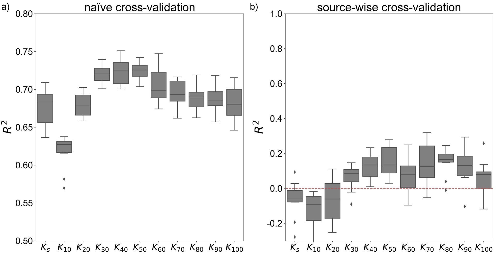
LGB model prediction performance for (a) the naïve and (b) the source-wise cross-validation schemes of the ten realisations of the nested training, testing and validation loop for each investigated supply tension, respectively. Note that the scales for the y-axes differ between (a) and (b).
Important predictors
Figure 18 illustrates Boruta feature selection frequencies as a measure for predictor importance for Ks and K100. Note that a lack of correlation between predictor and its SHAP value like for the soil organic carbon content in Figure 18b does not necessarily imply that the relationship was fundamentally shifting for each realisation of the ten-fold cross-validations. It may also mean that the relationship was stable but non-linear. Remember that correlations for categorical variables like the WRB soil type were related to Catboost-encoded values. They can only be properly interpreted with taking the encoding into account. The relationship between decoded WRB soil types and their SHAP and K100 values are shown in Figure 19.
The importance of individual predictors changed for Kh with supply tension, but converged to a stable set of predictors for drier conditions (Figure 20). The most important predictors for Ks (Figure 20a) were the longitude of the measurement location and cereals within the crop rotation implemented at the measurement site. For both we found it is difficult to explain why they should have a stronger impact on Ks than e.g. the bulk density. It is possible that the longitude encodes experimenter bias between researchers in the USA and Europe, the two global regions from where the majority of OTIM-DB data-entries stem. Alternatively, it may encode the more continental climate of North America as compared to Europe, under which then soils with different Kh had developed. Similar speculations may be undertaken to explain the impact of cereals in the crop rotation. However, we suspect that most of the predictors with large Boruta selection frequencies for estimating Ks rather expressed random bias in the OTIM-DB dataset, i.e. the seemingly high importance of these predictors was associated with artefacts from over-fitting. This view is supported by the fact that the LGB model was not able to predict Ks with R2 of more than zero.
The bulk density, in contrast, was likely a predictor that was assigned large importance due to its causal relationship with Kh. It showed up prominently among the most important predictors for supply tensions smaller than 50 mm (Figures 19a and 21). A large bulk density was always associated with a decrease in Kh. This reflects empirical knowledge. The correlation analyses in section XY likewise indicated the largest impact of bulk density on Kh near saturation. We therefore infer that the bulk density is a predictor whose usefulness for estimating Kh at and near-saturation is beyond doubt.
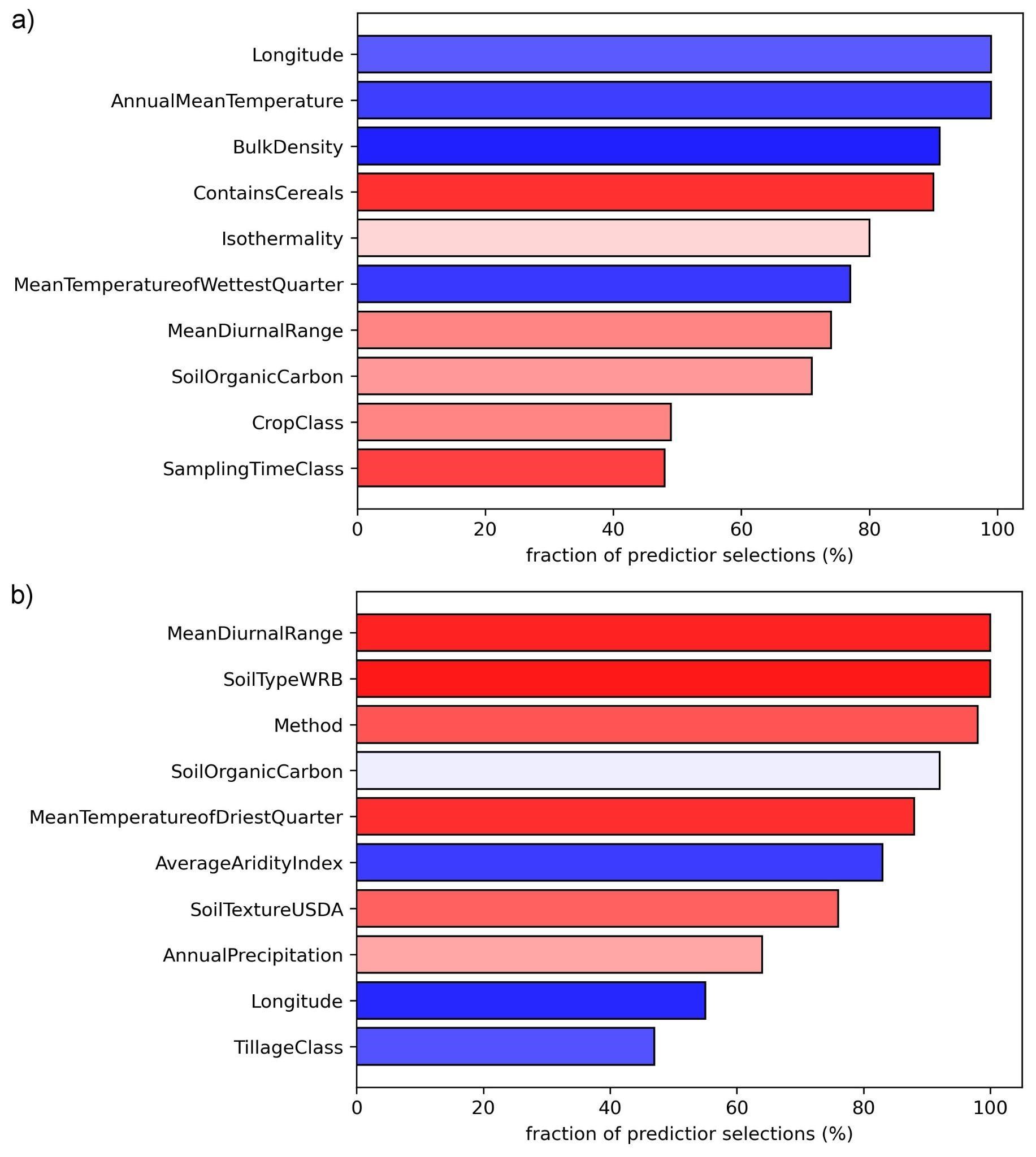
The ten most important predictors for (a) Ks, and (d) K100 resulting from the naïve cross-validation scheme. Red, white and blue colours indicate positive, absent and negative Pearson correlations of the predictors’ SHAP values with the respective Kh. The selection frequency refers to the Boruta feature selection.
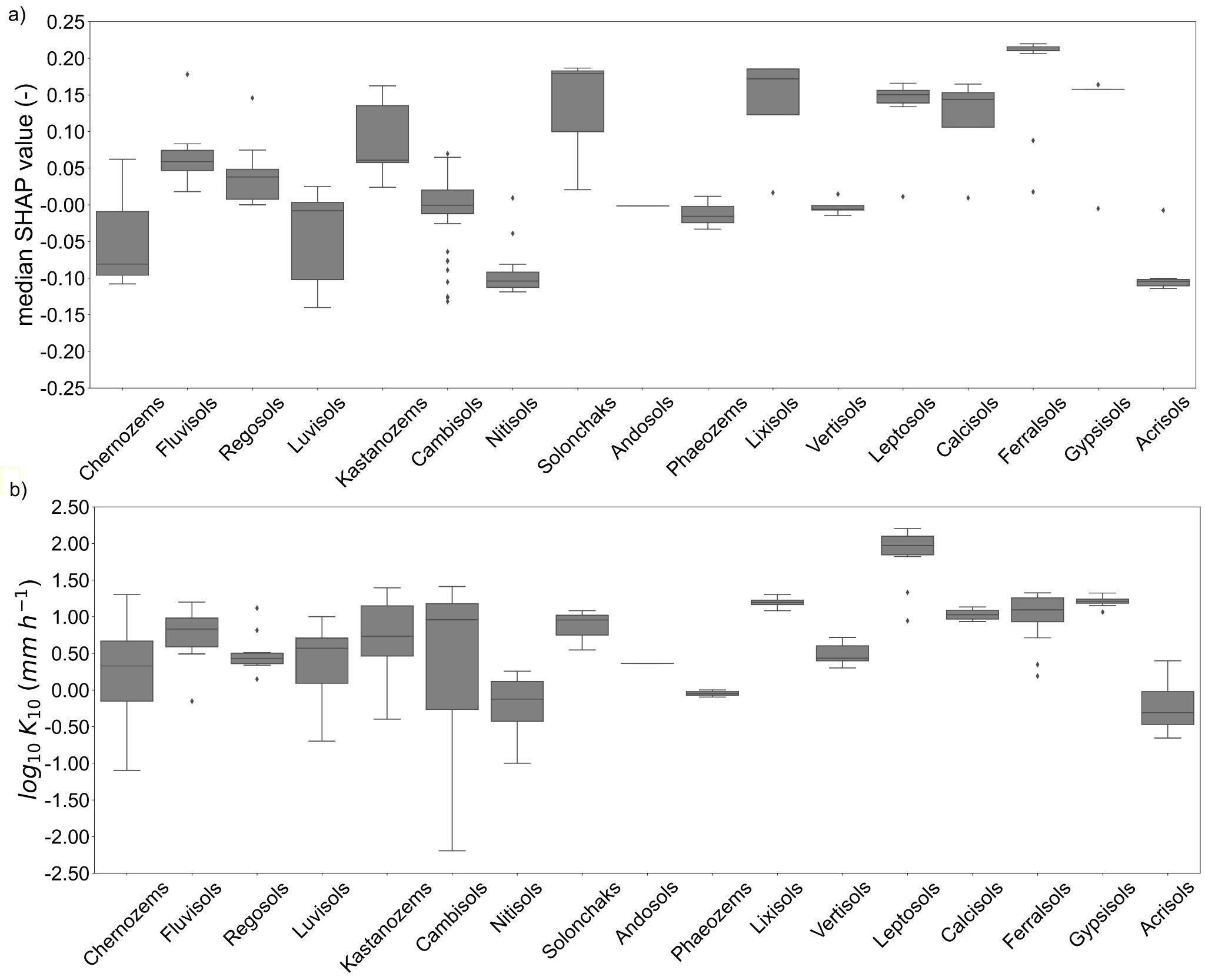
(a) SHAP values of individual WRB soil types and (b) the respective K100. Positive SHAP values means the predictor contributes positively to the prediction of K.
Notably, land use, tillage type, compaction or time of measurement only occasionally entered the lower ranks of the ten most frequently selected predictors, albeit they were shown to coincide with clear alterations in Kh in the meta-analyses (Section %s). Apparently, their impact was strongly dependent on the context, e.g. when comparing tilled with no-till arable fields. It may be that the rather simplistic design of our predictor importance analysis could not extract this context specific information. Using a simpler machine learning approach like a random forest may have had advantages in this respect, as Koestel & Jorda (2014), when using a random forest to predict the strength of preferential flow, were able to identify predictors that became only important under specific circumstances.
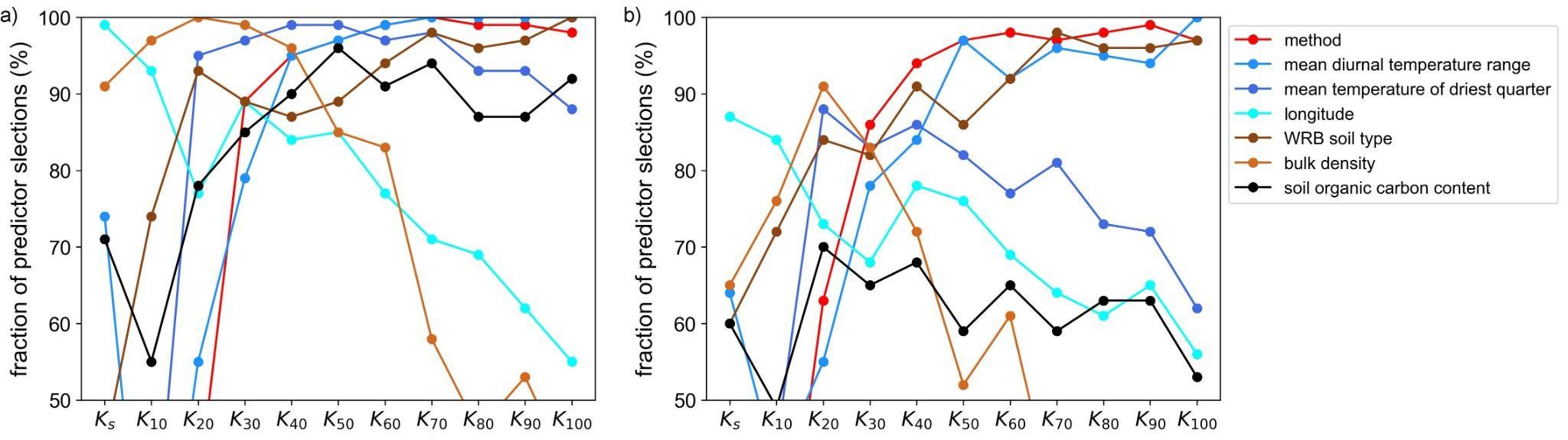
Selection frequency of some individual predictors in the Boruta feature selection for (a) the naïve cross-validation and (b) the source-wise cross-validation schemes.
At the dry end of the considered supply tension range, the mean diurnal temperature range, the method to convert infiltration rate to Kh, the WRB soil type and the USDA soil texture were the most important predictors (Figure 18b and Figure 20). The first two already had been discussed in the meta-analyses (Section %s). The mean diurnal temperature range showed the largest correlation with Kh for supply tensions larger than 10 mm. It is unclear what the reason for the large correlation is. Among the methods to convert infiltration rate to Kh, it is especially the ‘steady-state constant’ method that is known to overestimate Kh in the dry end of the here investigated tension range. As discussed, the impact of WRB soil type can only be understood with the aid of its relationship to Kh. Figure 19 illustrates that the respective SHAP values follow the K100 observed for individual soil types. This is in line with the positive correlation between WRB soil type SHAP values and K100 indicated in Figure 19b. It may be doubted if the association of K100 with specific soil types in OTIM-DB was representative for the general case. The large K100 for Leptosols may result from the fact that these soils often develop on coarse gravel. Also the low K100 for Acrisols are consistent with the low structural stability of this soil type. However, Nitisols are generally associated with large hydraulic conductivities, while the opposite was observed for the Nitisols in OTIM-DB. Whether WRB soil types are truly useful predictors for the near-saturated hydraulic conductivity needs to be investigated on a larger set of data.
Eventually, we want to mention that the soil organic carbon content was constantly among the ten most important predictors (see Figure 20). However, it always remained in the lower half of these lists. This may indicate that the soil organic carbon content is a predictor that is useful to further classify Kh after its value was already roughly estimated by more important predictors. Notably, the soil organic carbon content was positively correlated with Ks and negatively with K100, mirroring the correlations observed in the meta-analyses (see Section %s and discussions therein).
Conclusions of machine learning part
The LGB model trained in our study is not suited to serve as a pedotransfer function for the saturated and near-saturated hydraulic conductivity, because its prediction performance is clearly too low. The failure of developing a functioning pedotransfer function was most probably associated with i) a lack in suitability of the available proxy variables as predictors, ii) an insufficient amount of data points to estimate Kh using weak predictors and iii) experimenters’ bias. The Python code published in form of a Jupyter notebook alongside with this report may however be used to train LGB models tailored to new measurement sites if the models are spiked with a number measurements and meta-data from this new site.
The importance of predictors for Kh at and very close to saturation are probably not trustworthy, with exception of the bulk density. The most important predictors for Kh at the dry end of the investigated tension range are consistent with correlations observed in the meta-analyses and are predominantly backed by empirical knowledge. Our results support the conclusion of the meta-analyses part of our study that there is a need to investigate the reasons for the large observed correlations of climate variables like the mean diurnal temperature range or the mean temperature of the wettest quarter of the year with Kh. Context-specific relationships could barely be extracted using the LGB model predictor importance. At least, the absence of land use and soil management practises among the most important predictors indicate that, while they were shown in the meta-analyses to affect Kh, their impact is constraint to specific contexts, e.g. it is only observable when arable fields are considered.
General conclusions
We confirmed significant correlations between climate variables as well as the elevation above sea level with saturated and near saturated hydraulic conductivity. While it seems very likely that these variables influence soil physical properties, the exact underlying mechanisms need to be investigated in future studies. We found indications that specific soil management practises lead to changes in saturated and near-saturated hydraulic conductivities, which were increased under perennial cultures and decreased for no-till arable fields with annual crops and for compacted soil. Our data also confirmed that it is fundamental to take the time of the measurement after the last tillage operation into account to understand relationships between soil management and saturated and near-saturated hydraulic conductivity. Note that the management impacts turned out to be dependent on the pedo-climatic context, as they only could be observed if variations in the latter were ruled out. We also found that the data availability for tension-disk infiltrometer data was too scarce and riddled with too many gaps for detailed analyses of other soil management impacts, more specific pedo-climatic context dependencies and publication bias. Furthermore, we found indications that the available data was afflicted with experimenter bias. Altogether, it was not possible to predict saturated and near-saturated hydraulic conductivities from the available data for new sites, which echoes results of similar attempts to build respective pedotransfer functions. More measurements with better documented meta-data and better suited predictor variables would be needed for progress in this field. Studies quantifying soil structure evolution with respect to season, land use and soil management using X-ray imaging may turn out to provide useful information for more appropriate proxy variables for the saturated and near-saturated hydraulic conductivities.
- Larsbo, M., Koestel, J., & Jarvis, N. (2014). Relations between macropore network characteristics and the degree of preferential solute transport. Hydrology and Earth System Sciences, 18(12), 5255–5269. 10.5194/hess-18-5255-2014
- Klute, A., & Dirksen, C. (1986). Hydraulic conductivity and diffusivity: Laboratory measurements. In A. Klute (Ed.), Methods of soil analysis, Part 1 (second edition, Vol. 1, pp. 687–734). Soil Science Society of America, Inc.
- Angulo-Jaramillo, R., Vandervaere, J. P., Roulier, S., Thony, J. L., Gaudet, J. P., & Vauclin, M. (2000). Field measurement of soil surface hydraulic properties by disc and ring infiltrometers - A review and recent developments. Soil & Tillage Research, 55(1–2), 1–29. ://000088008800001
- Bouma, J. (1989). Using soil survey data for quantitative land evaluation. Advances in Soil Science, 9, 177–213. ://CABI:19891933076
- Van Looy, K., Bouma, J., Herbst, M., Koestel, J., Minasny, B., Mishra, U., Montzka, C., Nemes, A., Pachepsky, Y. A., Padarian, J., Schaap, M. G., Toth, B., Verhoef, A., Vanderborght, J., Ploeg, M. J., Weihermuller, L., Zacharias, S., Zhang, Y. G., & Vereecken, H. (2017). Pedotransfer Functions in Earth System Science: Challenges and Perspectives. Reviews of Geophysics, 55(4), 1199–1256. 10.1002/2017rg000581